A2. Electric Fields

Maitri Warusawithana

Section A: Sources and Fields

A2. Electric Fields

Sub Topics covered in this Module:

Introduction to Electric Fields
Electric Field of a Point Charge
Electric Field from Multiple Point Charges
Electric Field Lines
Electric Dipole
Electric Charge Density
Electric Field of Extended Charges

introduction to electric fields

In Module A1 we started to introduce a new concept that we called a “field”. There, in our discussion of electric charge, we stated that electric charge is a source that generates an electric field. Later (in Section D) you will see that electric fields can also be created without an electric charge as its source. But what exactly is an electric field? It is a vector quantity associated with every point in space—an abstract quantity with magnitude and direction that is related to its source (and the relative location of the source).

How do we know that such an abstract vector quantity that we call an electric field exists? How do we find the strength and direction of this electric field at a particular point in space? It turns out that such an electric field is experienced (felt) by another charged object (which we can call a “sensor”) placed at the point of interest. The “sensor” (a charged object) experiences a force due to the electric field at that point. Based on the force acting on this “sensor” we can determine both the magnitude and direction of the electric field vector at this point. Note that a neutral object is not a good “sensor” of the electric field as it will not experience a net force due to an electric field at its location.

Tidbit:

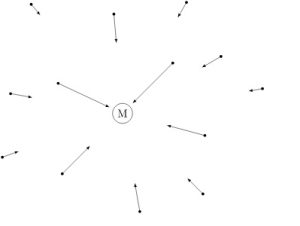
Figure A2.1: Field vectors at different points due to earth’s gravitational field.

Consider the earth’s gravitational field for example. The mass of the earth is the source that generates this gravitational field. This gravitational field has a strength and a direction at every point in space, be it at the top of mount Everest or at the foot of the Eiffel Tower in Paris, or at any other point in space. Since another mass will interact with (experience) this gravitational field, we can use it as a “sensor” to find the gravitational field vector at each of these points. We shall call this “sensor” a test mass ( $m_t$ ). It is important to make sure that this test mass is small and that it does not significantly perturb the gravitational field at the point of interest. By measuring the strength and direction of the gravitational force on the test mass ( $\vec{F}_{\vec{g}_{\vec{r}},m_t}$ ) the gravitational field vector ( $\vec{g}_{\vec{r}}$ ) can be determined at the location ( $\vec{r}$ ) the test mass is placed. Figure A2.1 shows a sketch of earth’s gravitational field vectors at different points.

$\vec{g}_{\vec{r}} = \frac{\vec{F}_{\vec{g}_{\vec{r}},m_t}}{m_t}$

The abstract concept of an electric field is similar to the abstract concept of a gravitational field. They are abstract quantities that permeate space, quantities that have both a magnitude and a direction. In the case of an electric field, to determine the electric field vector at a point of interest we need a test charge to act as a “sensor” of the electric field. This test charge must be small such that it does not perturb the electric field at the point of interest. Moreover, since we have two flavors of charge that we called “positive” and “negative”, we must pick one flavor for our test charge and stick to this flavor so that the electric field is consistently defined in terms of our test—charge—convention. We shall pick the convention that our test charge is always a small positive charge.

With a positive test charge as our convention, we can now explore the electric field at any point ( $\vec{r}$ ) due to a source that generates an electric field. To do this, we take on a definition similar to the definition that we used to find the gravitational field (see above). That is, the electric field ( $\vec{E}_{\vec{r}}$ ) at the point of interest ( $\vec{r}$ ) is the force ( $\vec{F}_{\vec{E}_{\vec{r}}, q_{_t}}$ ) acting on the test charge placed at that point ( $\vec{r}$ ) divided by the test charge ( $q_{_t}$ ).

$\vec{E}_{\vec{r}} = \frac{\vec{F}_{\vec{E}_{\vec{r}}, q_{_t}}}{q_{_t}}$

Electric field of a point charge

Let us first consider a charged object as our source where the entire charge, $Q$ , of the object can be assumed to be localized to a point—we call this a point charge—a seemingly unrealistic simplification that makes for a great textbook example, but nevertheless very instructive and applicable when finding the electric field of more complicated charge distributions as you shall see later. We can find the magnitude of the electric field at point $P$ (with position vector $\vec{r}_{_{P}}$ ) due to this point source charge, $Q$ (located at position vector $\vec{r}_{_0}$ ) based on two observations:

1. that the force on a test charge placed at point $P$ is directly proportional to the strength of the point source charge, $Q$ . Since the electric field ( $\vec{E}$ ) at the location of the test charge is related to the force on the test charge,

$|\vec{E}| \propto Q$

2. that the force on a test charge placed at point $P$ (and thus the electric field at point $P$ ) is inversely proportional to $|\vec{r}_{_P}-\vec{r}_{_0}|^2$ , the square of the distance from the point source charge, $Q$ , to point $P$ .

$|\vec{E}| \propto \frac{1}{|\vec{r}_{_P}-\vec{r}_{_0}|^2}$

Combining these proportionalities, we find that

$|\vec{E}| \propto \frac{Q}{|\vec{r}_{_P}-\vec{r}_{_0}|^2}$

Let $\vec{r}=\vec{r}_{_P}-\vec{r}_{_0}$ be the position vector of point $P$ with respect to the location of the source charge $Q$ , see Figure A2.2. Then,

$|\vec{E}_{\vec{r}}| \propto \frac{Q}{|\vec{r}|^2}$

It turns out that the proportionality constant is given by $\frac{1}{4\pi\varepsilon_0}$ , where $\varepsilon_0$ is a fundamental constant known as the permittivity of free space

Permittivity of free space

$\varepsilon_0=8.8541878128\times10^{-12} \frac{C^2}{Nm^2}$

$k=\frac{1}{4\pi\varepsilon_0}\approx8.99\times10^9 \frac{Nm^2}{C^2}$

Which gives us:

(1) $\begin{equation*} |\vec{E}_{\vec{r}}|=\frac{kQ}{|\vec{r}|^2}\end{equation*}$

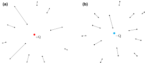
The direction of the electric field at point $P$ can be determined by the direction of the force experienced by the test charge when placed at point $P$ . Since by convention our test charge is positive, if the point source charge, $Q$ , is positive, the force on the test charge will be a repulsive force that points away from the source charge. On the other hand, if the point source charge, $Q$ , is negative, the force on the test charge will be an attractive force that points toward the source charge. The electric field vector can therefore be expressed as:

(2) $\begin{equation*} \vec{E}_{\vec{r}}=\frac{kQ}{|\vec{r}|^2} \hat{r}\end{equation*}$

where $\hat{r}=\frac{\vec{r}}{|\vec{r}|}$ is a unit vector that points in the direction from the point source charge, $Q$ , to point $P$ .

By moving the test charge to different points in space, the electric field vectors at each point can be determined. See Figure A2.3.

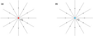
Figure A2.3: Electric field vectors at different points in space due to a point charge. (a) Due to a positive point source charge. (b) Due to a negative point source charge.

To visually represent electric fields we can also use electric field lines. Field lines are a graphical way to represent a “vector field”. The electric field line diagrams for positive and negative point charges are shown in Figure A2.4. Note that this is different to the diagrams representing field vectors. See section below on electric field lines for more information.

Figure A2.4: Using electric field lines to represent the electric field due to a point source charge. (a) For a positive point source charge. (b) For a negative point source charge.

Electric Field from Multiple Point Charges

Equation 2 gives the electric field vector at a point with position vector $\vec{r}$ relative to point charge $Q$ . Let’s extend this to find the electric field at a given point when multiple point charges are present in the region. In this case we will first need to find the individual electric fields at the given point due to each point charge using equation 2. We can then take the vector sum of these individual electric field vectors to find the net electric field at the point of interest. We call this superposition of vectors, and is expressed in equation 3 below.

(3) $\begin{equation*} \vec{E}_{net}=\displaystyle \sum\limits_{n=1}^{N}} \vec{E}_n=\vec{E}_1+\vec{E}_2+\vec{E}_3+\ldots+\vec{E}_N\end{equation*}$

The process above can be carried out in four steps:

*1. Using equation 1 find the magnitude of each electric field at the point of interest due to each of the charges (ignore the sign of the charges).

*2. Determine the direction of each field at the point of interest based on the sign of each charge. Recall that the interaction between each point charge and a hypothetical (positive) test charge placed at the point of interest will give the direction of each electric field.

3. Draw a field vector diagram showing each electric field at the point of interest.

4. Determine the vector sum of all the individual fields.

*Note: the first two steps can be done in any order.

Concept Check

Question A9

Refer to the following figure to answer the question:

Rendered by QuickLaTeX.com

Concept Check

Question A10

Refer to the following figure to answer the question:

Rendered by QuickLaTeX.com

Concept Check

Question A11

Refer to the following figure to answer the question:

Concept Check

Question A12

Refer to the following figure to answer the question:

Rendered by QuickLaTeX.com

Electric field lines

Field lines are a graphical way to represent a “vector field”. The direction of the vector field at any point in space is indicated by the direction of the field line at that point. The density of field lines in a region of space provide information on the strength of the vector field in that region. Features specific to electric field lines are listed below:

The electric field at any point is tangent to the electric field line passing through that point.

The denser the electric field lines are, the stronger the electric field in that region.
Two field lines never cross.
Electric field lines start and end at a source or they appear to extend out to infinity. Based on our convention, electric field lines start from a positive charge and end at a negative charge.

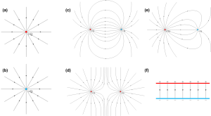
Figure A2.5 shows examples of electric field lines for different charge distributions:

Figure A2.5: Electric field lines for different charge distributions. (a) For a positive point charge. (b) For a negative point charge. (c) For an electric dipole (a positive and negative point charge of equal magnitude). (d) For two positive point charges of equal magnitude. (e) For a positive and a negative point charge of unequal magnitude. (f) For parallel plates charged positive and negative.

Concept Check

Question A13

***Under construction***

Refer to the following figure to answer the question:

Concept Check

Question A14

***Under construction***

Refer to the following figure to answer the question:

Electric dipole

Two opposite charges of equal magnitude that are spatially separated, forms an electric dipole. Such a configuration of charge is commonly encountered in nature. Some naturally occurring materials are made up of electric dipoles, for example, water. Water molecules are permanent dipoles. See Figure A2.6. Electric dipoles can also be formed in certain neutral materials by inducing a spatial separation of positive and negative charge. See Figure A2.7. In this section we are interested in the electric field generated by an electric dipole. But, we will further explore electric dipoles later in the text: in comparison to magnetic dipoles (in Section A3), in electronic materials like dielectrics and ferroelectrics (in Section C4), and in studying their equilibrium and dynamics (in Section E1).

Rendered by QuickLaTeX.com — Figure A2.6: In a water molecule, H₂O, the electron of each hydrogen atom that participates in bonding spends more time near the oxygen atom giving each hydrogen atom a slight positive charge and the oxygen atom a slight negative charge. This separation of charge makes a water molecule act as a permanent dipole.

Figure A2.7: A charged rod is used to flip a magazine page. The charged rod polarizes the sheet of paper causing a separation of charge in the paper (at the nanometer scale) resulting in induced dipoles in the sheet of paper.

The spatial separation of positive and negative charge in a dipole inherently results in an electric field. We can find this electric field generated by the dipole at any point in space using the technique of superposition discussed above. i.e. considering the dipole as two point charges (positive and negative), individually finding the electric field vectors at the point of interest due to each charge, and finally carrying out vector addition to find the net electric field. Before we carry out a mathematical derivation, however, it is instructive to note that the dipole as a whole has a net neutral charge (equal positive and negative charges). As such, the electric field very far away from the dipole (where the separation between the charges is inconsequential compared to the distance from the dipole to the point of interest) must be zero. In fact, we will see that the electric field of a dipole drops off as $\mathsf{\nicefrac{1}{distance^3}}$ . i.e. given the net-neutral charge of a dipole, the electric field of a dipole decreases more quickly with increasing distance than the electric field due to a single point charge which decreases only as $\large{\mathsf{\nicefrac{1}{distance^2}}}$ .

Let us first consider a point on the axis of the dipole such as point $P$ as indicated in Figure A2.8, which is a distance z from the center of the dipole. Given the spatial separation, $d$ , between the $+Q$ charge and the $-Q$ charge of the dipole, we can find the distances

$r_+=|\vec{r}_{_P}-\vec{r}_{_{0_+}}|=|z \hat{z}-\frac{d}{2} \hat{z}| = z-\frac{d}{2}$

$r_-=|\vec{r}_{_P}-\vec{r}_{_{0_-}}|=|z \hat{z}+\frac{d}{2} \hat{z}| = z+\frac{d}{2}$

based on our convention for $\vec{r_{_P}}$ and $\vec{r}_{_0}$ as shown in Figure A2.2.

Considering the $+Q$ charge and $-Q$ charge as point charges, we can find the individual electric fields, $\vec{E}_{p_+}$ and $\vec{E}_{p_-}$ , at point $P$ due to each of the charges

(4) $\begin{equation*} \vec{E}_{p_+}=\frac{kQ}{r_{+}^{ 2}} \hat{z}=\frac{kQ}{\left(z-\frac{d}{2}\right)^{2}} \hat{z}\end{equation*}$

(5) $\begin{equation*} \vec{E}_{p_-}=\frac{kQ}{r_{-}^{ 2}} (-\hat{z})=\frac{kQ}{\left(z+\frac{d}{2}\right)^{2}} (-\hat{z})\end{equation*}$

Then using the superposition principle, we find the net electric field at point $P$ ,

(6) $\begin{equation*} \vec{E}_p=kQ\left[\frac{1}{\left(z-\frac{d}{2}\right)^{2}}-\frac{1}{\left(z+\frac{d}{2}\right)^{2}}\right]\hat{z}\end{equation*}$

Note that in most cases we are interested in the electric field at distances from the dipole that are much larger compared to $d$ given that electric dipoles are typically microscopic and in most cases nanoscopic in nature. i.e. the separation, $d$ , between the positive and negative charge of a dipole is very small—on the order of micrometers (10^-6 m) or nanometers (10^-9m). Therefore in the limit that $z>>d$ , we can simplify and approximate equation 6 and express the electric field at point $P$ as,

(7) $\begin{equation*} \vec{E}_p=\frac{2kQd}{z^3}\hat{z}\end{equation*}$

We define the quantity, $Qd\hat{z}$ , in the numerator as the dipole moment vector, $\vec{p}$ , which is a constant for the particular dipole. The direction of the dipole moment vector is the direction pointing from the negative charge to the positive charge of the dipole.

(8) $\begin{equation*} \vec{p}=Qd\hat{z}\end{equation*}$

Using the dipole moment vector, $\vec{p}$ , we can express the electric field at point $P$ as:

(9) $\begin{equation*} \vec{E}_p=\frac{2k\vec{p}}{z^3}\end{equation*}$

As mentioned before, we see that the electric field of a dipole (in the limit $z>>d$ ) drops off as $\frac{1}{z^3}$ .

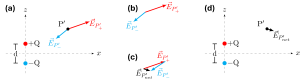
Finding the electric field of the dipole at any general point, $P'$ , can be accomplished using the same process. This is illustrated in Figure A2.9. The first step is to find the individual electric fields, $\vec{E_P_+'}$ and $\vec{E_P_-'}$ , at point $P'$ due to each charge. Then the net electric field at $P'$ can be obtained using the superposition principle (vector addition), which is graphically represented in Figure A2.9. Given the different directions of the two vectors, for any general point, $P'$ , the vector addition can be a little involved, but nevertheless can be accomplished to find the electric field of the dipole at any general point. Refer to Figure A2.5(c), electric field lines for a dipole, to visualize the electric field at any general point due to a dipole.

Figure A2.9: Finding the electric field at a general point (P’) due to an electric dipole. (a) Electric field vectors at point P’ (not on dipole axis) due to +Q and -Q charges of an electric dipole with separation d. (b) Field vector diagram. (c) Finding the net electric field using vector addition. (d) Net electric field at point P’ due to the electric dipole.

Electric charge density

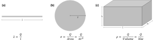
In real life, we have extended objects, not point charges. When considering extended objects with a uniform or regular charge distribution, it is useful to understand the concept of charge density. An extended object, by definition, is 3-dimensional. But, based on the shape of the object, sometimes the object’s dimensionality can be reduced to two dimensions or one dimension without loss of generality just for the purpose of solving the problem. A meterstick, for example, where the charge is spread out along its length, can be considered 1-dimensional. It still has a width and a thickness to it, making it a 3-dimensional object. But if we can neglect any variation in the charge across its width and its thickness, then there is no loss of generality in considering it a 1-dimensional object. Similarly, a charged pancake can be considered 2-dimensional if any variation in the charge across its thickness can be neglected.

A 3-dimensional object will have a volume charge density, a charge that is distributed based on volume and denoted by the greek letter rho, $\rho$ (with SI units $C/m^3$ ). Similarly, an object that can be considered 2-dimensional will have an areal charge density, a charge that is distributed based on area and denoted by the greek letter sigma, $\sigma$ (with SI units $C/m^2$ ). Likewise, an object that can be considered 1-dimensional will have a line charge density, a charge that is distributed based on the length and denoted by the greek letter lambda, $\lambda$ (with SI units $C/m$ ). See Figure A2.10 for examples of three objects each with a uniformly distributed $+Q$ charge.

Figure A2.10: Examples of three objects with a uniformly distributed +Q charge. (a) Line charge density. (b) Surface charge density. (c) Volume charge density.

Electric Field of extended charges

So far, we have only considered the electric field of point objects. Using the knowledge we have gathered, specifically the three aspects listed below, we can now try to determine the electric field of more realistic extended objects.

The inverse-square relationship that governs the electric field of a point charge
The superposition principle for vector addition used to find the electric field due to multiple point charges
Our knowledge of differential calculus

Note:

Calculating the electric field exactly of any odd, irregularly shaped object (or an object with a regular shape but an irregular charge distribution) is a horrendous problem. If, in the real world, you encounter a situation where the electric field of such an irregular object needs to be found, you will have to proceed by first making some approximations (to convert it to a regular-shaped object with a regular charge distribution) and then find the electric field of this approximate shape. Also note that in some real-world instances, a simple fermi calculation to find an order-of-magnitude estimate could be all that is needed, instead of an exact calculation.

In what follows, we outline a process to exactly calculate the electric field at a point due to a regular-shaped object with a uniform or regular (but non-uniform) charge distribution.

Hypothetically break the extended object into small, “elemental” pieces. It is important to consider the shape and symmetry of the object as you break it into elemental sections. An elemental section is one that is small enough that it can be considered a point object.
Find an expression for $\textbf{\textit{dq}}$ : Select one of these elements as a general, representative section. Assume this elemental section has a charge $dq$ . Express $dq$ either as a fraction of the overall charge of the object or as a function of the charge density based on the information given.
Find the electric field (magnitude and direction) at the point of interest due to this selected elemental charge, $\textbf{\textit{dq}}$ . Here $dq$ will be considered a point charge and the inverse square relationship will be used. A reference frame (coordinate system) should be picked so that this electric field due to $dq$ can be expressed in terms of this reference frame.
Carry out an integral to find the net electric field vector: Use superposition principle to carry out a vector sum of all the electric field contributions at the point of interest due to each elemental charge. Since we are considering the limit that each elemental section tends to a point, this turns out to be an infinite vector sum and we will need to apply differential calculus (integration) to perform this infinite sum.

Example A2.1:

A thin charged rod placed on the x axis as shown in the figure has a non-uniform negative line charge density that increases from $a$ to $b$ , (with the left end of the rod having zero charge) given by $\lambda(x)=C(x-a)^2$ , where $C$ is a negative constant with units $C/m^3$ . Find the electric field at the origin due to this charged rod.

Solution

Example A2.2:

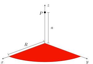
A thin quarter-circular plastic plate of radius $R$ is uniformly charged with a total positive charge $+Q$ . i.e. the charge $+Q$ is uniformly distributed over the surface area of the plate. Find the electric field at point $P$ which is a height $a$ right above the corner of the plate as shown in the figure.

[insert figure]

Solution ***Under construction***

Continue to A3

License

Icon for the Creative Commons Attribution 4.0 International License

introduction to electric fields

Electric field of a point charge

Electric Field from Multiple Point Charges

Electric field lines

Electric dipole

Electric charge density

Electric Field of extended charges

License

Share This Book