In this section we will focus on differential equations that model climate change. Now compared to sophisticated climate models used by climate scientists, this is just a toy model and doesn’t cover all the complexities of real climate. However, it does show how feedback loops can amplify the effects of climate change.
Photo by Ian Barbour
In terms of global earth temperature, what greenhouse gas is responsible for trapping the most heat? You may be surprised to learn that it is H[latex]_2[/latex]O, not CO[latex]_2[/latex]. Water vapor is a more effective greenhouse gas than carbon dioxide, and there is a lot more of it too. So why don’t more people talk about H[latex]_2[/latex]O in regards to global warming? It’s because the amount of H[latex]_2[/latex]O is not a driving force behind climate change. The H[latex]_2[/latex]O is dependent on temperature to begin with. Since you can’t increase the H[latex]_2[/latex]O without increasing temperature, you can’t use H[latex]_2[/latex]O to increase temperature. However, that doesn’t mean H[latex]_2[/latex]O can be ignored either.
Consider the following set of differential equations. [latex]T(t)[/latex] is the global temperature, [latex]W(t)[/latex] is the amount of water, and [latex]C(t)[/latex] the amount of carbon.
\begin{align*}
\frac{d}{dt} T & = c – d T+ e W + f C \\
\frac{d}{dt} W & = a (gT – W) \\
\frac{d}{dt} C & = b
\end{align*}
Okay, let’s go through the steps.
- Understand what each variable is measuring with correct units.
There are no units listed in the problem, so we will make up some reasonable guesses for what they are. Anyway, [latex]t[/latex] is a measure of time as usual, we could say measured in years after some starting date. [latex]T(t)[/latex] is the global temperature, we will say measured in Celsius. [latex]W(t)[/latex] is the average concentration of water vapor globally at time [latex]t[/latex], and [latex]C(t)[/latex] is similar for CO[latex]_2[/latex]. We will assume [latex]W(t)[/latex] and [latex]C(t)[/latex] are measured in parts per million, or ppm. Then we have [latex]\frac{d}{dt} T[/latex] is how fast the temperature is changing globally (in degrees Celsius per year), [latex]\frac{d}{dt} W[/latex] is the change of water concentration (in ppm per year), and [latex]\frac{d}{dt} C[/latex] is the change in CO[latex]_2[/latex] (in ppm per year). Note that while I “guessed” the units for [latex]t[/latex], [latex]W(t)[/latex] and [latex]C(t)[/latex], the units for a derivative are forced from those choices, so I can’t just make up new units for say [latex]\frac{d}{dt} W[/latex]. See this chapter on interpreting the derivative for more information.
So what are [latex]a, b, c, d, e, f, g[/latex]? Well, we’ll talk about these more in the next step but they are basically parameters that relate how much of an effect various quantities have on each other.
- Write down what relationship the differential equation is describing in common, no-nonsense language.
Let’s start with the simplest equation: [latex]\frac{d}{dt} C = b[/latex]. This is just saying that carbon is increasing (or decreasing) at a constant rate [latex]b[/latex]. This tells us what [latex]b[/latex] is as well; assuming [latex]b[/latex] is positive, it’s how fast we’re putting carbon into the atmosphere.
The next simplest equation is [latex]\frac{d}{dt} W = a (gT - W)[/latex]. Ignoring [latex]a[/latex] and [latex]g[/latex] for a second, this tells us that water vapor increases at a rate that looks like the difference between temperature and water vapor. So a hot and dry atmosphere will tend to get wetter, while a cool or damp atmosphere might mean a negative difference so it would get less wet. The values of [latex]a[/latex] and [latex]g[/latex] affect the severity of these trends.
Finally, let’s look at the more complicated equation: [latex]\frac{d}{dt} T = c - d T+ e W + f C[/latex]. Let us break that down into two pieces, starting with [latex]c - dT[/latex]. Assuming [latex]c[/latex] is positive, the [latex]c[/latex] is basically a constant source of temperature increase. However, as the temperature increases, we see that the [latex]-dT[/latex] term will tend to cool things off. We will see in the next step what these terms really mean. But for now, let’s move on to [latex]+eW + fC[/latex]. This is saying that the bigger [latex]W[/latex] and [latex]C[/latex] are, the hotter the earth will get.
- Explain why those relationships seem to make sense.
We just got done thinking about the equation [latex]\frac{d}{dt} T = c - d T+ e W + f C[/latex], so let’s start there. Let’s focus on [latex]c - dT[/latex]. Why are these terms here influencing temperature? Well, we said [latex]c[/latex] was a constant source of temperature increase — does that ring a bell? Yes, it’s the sun! Ignoring other effects, we will continue to absorb solar energy until we are hotter than Venus. So hopefully there is something that will cool us off. In this equation it is the term [latex]-dT[/latex]. Why is this term here? Well, it turns out the hotter the earth gets, the more heat energy will be radiated away. We don’t generally see this energy with our eyes, because it is infrared, but it’s there. This [latex]c - dT[/latex] is the basic energy balance that determines the temperature of the earth. A similar equation would hold true for any planet.
However, to this, we add [latex]+eW + fC[/latex]. Why? That’s right — water and carbon are greenhouse gases, so the more [latex]W[/latex] and [latex]C[/latex], the hotter the earth will tend to get. Now technically, these are really just absorbing that infrared energy from the earth, so they are not actually separate from the [latex]-dT[/latex] term, but for simplicity I’ve just listed them as separate terms. This is one of many simplifications in this model that a real climate model would correct. It’s important to note at this point that, even though carbon is the driver behind global warming, it’s actually the water that is the better greenhouse gas and much more prevalent. Because of this, the [latex]e[/latex] term should be much larger than the [latex]f[/latex] term.
Let’s focus now on the [latex]\frac{d}{dt} W = a (gT - W)[/latex] equation. We already said that this equation implies that hot and dry air will tend to absorb more water, while cool and damp air would lose water. This makes sense since hot air just holds more water. Also, the hot air will heat the oceans causing evaporation.
Finally, why do we have the equation [latex]\frac{d}{dt} C = b[/latex]? Well, the amount of carbon in the atmosphere is a very complex system. But for simplicity we can say it is increasing at a constant rate [latex]b[/latex], due mostly to humanity burning fossil fuels.
Okay, now we understand some things about these differential equations, what do they tell us? For this, we will turn to computers to create some graphs for us. These graphs are all solutions to the differential equations. And while these graphs won’t perfectly depict reality, they will show us some aspects of climate change you might not realize. We will use this website that graphs the solution for us. It looks like this:
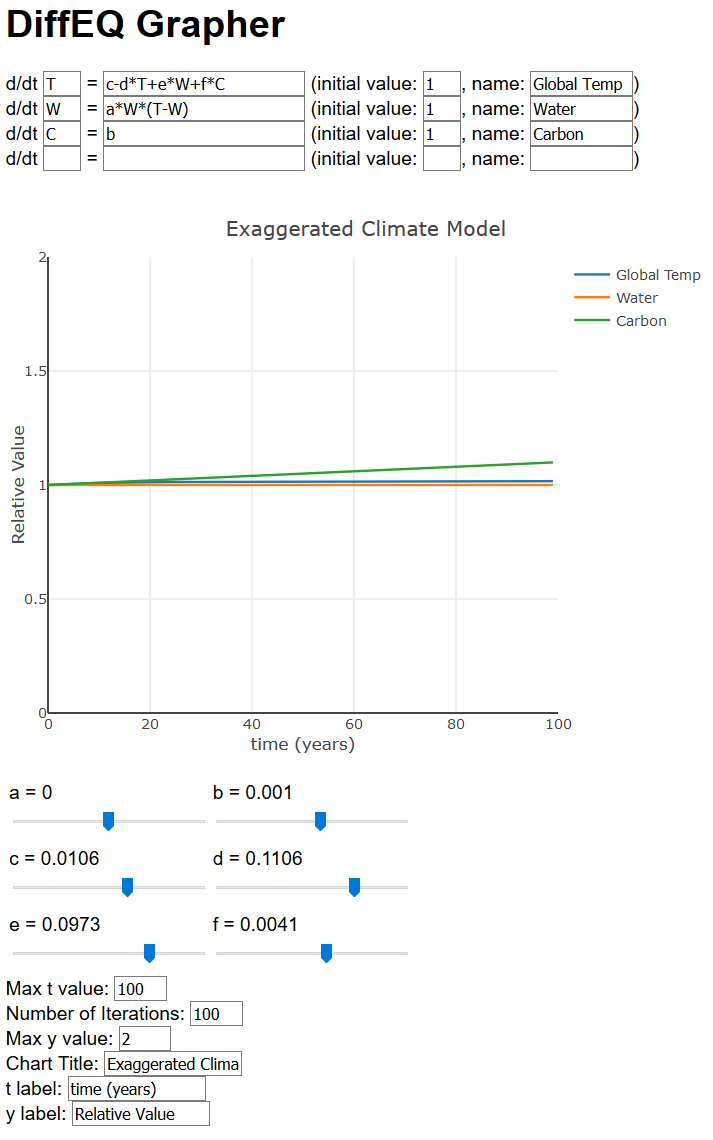
Let’s take a closer look at that graph. Note we have [latex]a = 0[/latex], [latex]b = 0.001[/latex], [latex]c = 0.01[/latex], [latex]d = 0.1[/latex], [latex]e = 0.1[/latex], and [latex]f = 0.004[/latex]. Notice that [latex]f[/latex] is much smaller than [latex]e[/latex], reflecting how much less of an effect carbon has compared to water.
Okay, not a lot happening yet. But you can start to get familiar with the graph. First, you’ll note that Global Temperature, Water, and Carbon levels are all around [latex]1[/latex]. Note that does not mean the temperature is [latex]1^\circ[/latex] C, or that Carbon is [latex]1[/latex] ppm. Instead this represents some sort of “relative” value of these quantities compared to normal. This makes it easier to put these things on the same graph. So [latex]1[/latex] represents normal, [latex]2[/latex] would be twice normal, [latex]0.5[/latex] would be half of normal, and so on.
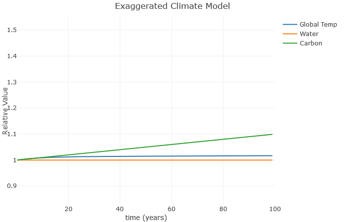
The amount of carbon in the atmosphere related to the [latex]b[/latex] value. So if I increase this from [latex]0.001[/latex] to about [latex]0.02[/latex], we see the change in the graph below.
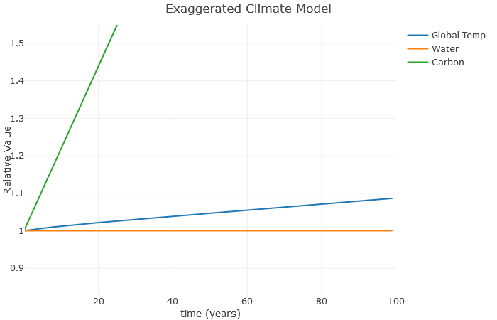
Now the carbon is taking off, but not much is happening to the global temperature. Why is this? Well, notice we set [latex]a = 0[/latex]. This has the effect of keeping the water value constant, even though in reality it would increase as the temperature increases. So let’s see what happens when we set [latex]a = 0.1[/latex]:
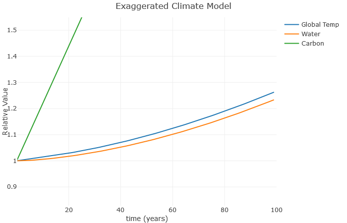
Now we can see how the temperature increases the water vapor, which furthers increases the temperature, which further increases the water vapor, and so on. This is a classic example of a climate feedback loop. The end result is a much higher global temperature with the same basic increase in carbon. This is consistent with more advanced models, which show that water roughly doubles the effect of carbon. Note that I don’t expect a 25% increase in temperature over the next [latex]100[/latex] years – this is exaggerated to illustrate the relationships.
A couple more things: Suppose we don’t increase carbon anymore, but still have that water vapor effect. What happens? Here, I’ve left [latex]a[/latex] at [latex]0.1[/latex], but reduced [latex]b[/latex] to [latex]0[/latex].
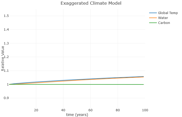
Clearly, this is much better than when we were increasing carbon so fast. However, notice there is still an increase in temperature. That’s because these feedback loops continue to operate even after we stop increasing carbon. As a result, scientists expect global temperatures to rise for several decades even if we manage to become carbon neutral as a planet.
Finally, the worst-case scenario is as follows. It has the same settings as the previous example, just with [latex]e[/latex] (the effect of water vapor) increased 10%
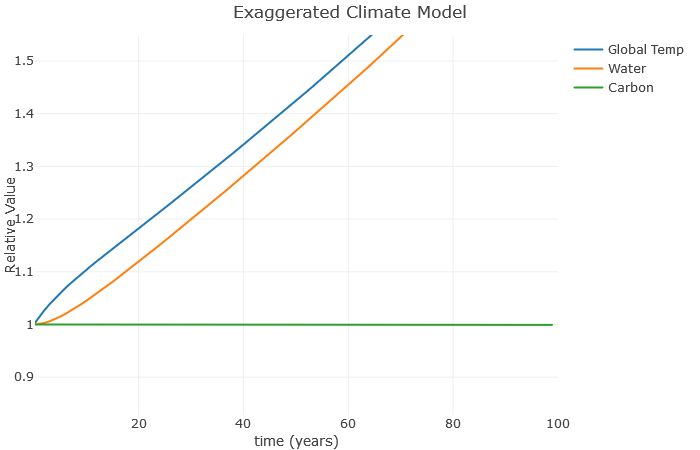
This is the “runaway greenhouse effect”, where a feedback loop gets out of control, and even with no additional carbon the temperature increases to the point where the seas boil away. Most scientists think this isn’t possible for earth even with large amounts of additional carbon, but with the right conditions this sort of thing is possible. Scientists think this is what happened to Venus hundreds of millions of years ago.
Please feel free to play around with the model yourself!
