Purpose: To be introduced to the concept of modeling with differential equations

In this project, you’ll choose a well-known differential equation model from biology, try to understand the differential equations, and explore graphical solutions.

Choose one of the following topics:

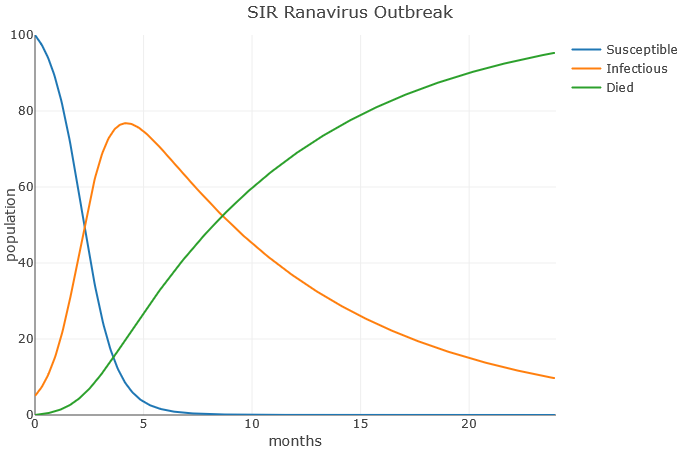
• SIR ranavirus model. Ranavirus is a disease that affects reptiles, amphibians, and fish; “Ranavirus is believed to be the cause of several recent mass mortality events in amphibian populations across the globe” (link). Given a population, let [latex]S(t)[/latex] be the number of frogs suseptible to ranavirus, let [latex]I(t)[/latex] be the number of frogs currently infected with the disease, and let [latex]R(t)[/latex] be the number of frogs that have died. Note that at any time, [latex]S(t) + I(t) + R(t)[/latex] is the equal to the total population.Then
  \begin{align*}
  \frac{dS}{dt} & = -a S(t) \cdot I(t) \\
  \frac{dI}{dt} & = a S(t) \cdot I(t) – b I(t) \\
  \frac{dR}{dt} & = b I(t)
  \end{align*}
  Here, [latex]a[/latex] and [latex]b[/latex] are unknown parameters that affect the dynamics of this problem.

  Click here for the DiffEQ grapher for the Ranavirus SIR model.

  

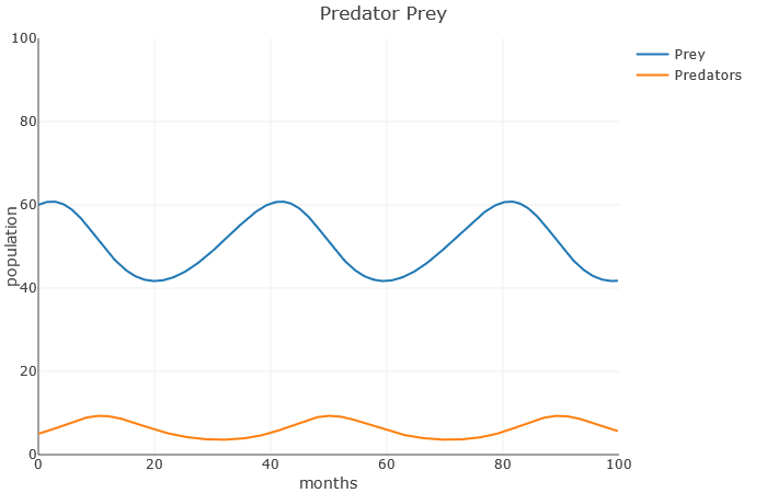
• Lotka-Volterra equations for simple modeling of predator and prey dynamics, such as the moose and wolf populations in Isle Royale National Park (link). Given [latex]M[/latex] is a population of prey (Moose), and [latex]W[/latex] is the population of predators (wolves), we have
  \begin{align*}
  \frac{dM}{dt} & = a M(t) – b M(t) \cdot W(t) \\
  \frac{dW}{dt} & = – c W(t) + d M(t) \cdot W(t)
  \end{align*}
  Here, [latex]a[/latex], [latex]b[/latex], [latex]c[/latex], and [latex]d[/latex] are unknown constants, but they are parameters that affect the interaction between the two species.

  Click here for the DiffEQ grapher for the Lotka-Volterra equations.
  

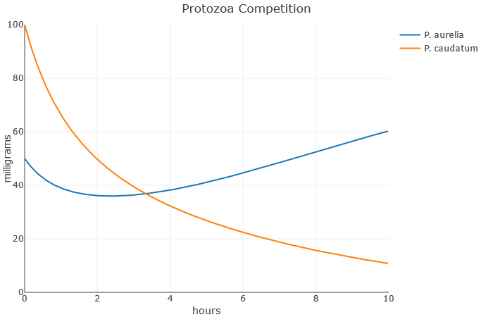
• Protozoa Competition: Paramecium aurelia and Paramecium caudatum are two species of single-celled protozoa, which were studied by G.F. Gause when he formulated his famous Competition exclusion principle (link). Let [latex]A(t)[/latex] be milligrams of Paramecium aurelia, and [latex]C(t)[/latex] be milligrams of Paramecium caudatum. Suppose [latex]A[/latex] and [latex]C[/latex] satisfy:
  \begin{align*}
  \frac{dA}{dt} & = a A(t) – b(A(t) + C(t)) A(t) \\
  \frac{dC}{dt} & = c C(t) – d(A(t) + C(t)) C(t)
  \end{align*}
  Here, [latex]a, b, c, d[/latex] are the parameters that affect this problem.

  Click here for the DiffEQ grapher for the Protozoa equations.

  

Once you’ve chosen a topic, here is what to do:

1. Follow the steps from the section on understanding differential equations to understand what the differential equation is saying.
2. Give an example: what are some realistic numbers for the differential equation? What do they tell you?
3. Using the supplied “DiffEQ” webpage, explore graphical solutions to the differential equation.
   1. What do the parameters [latex]a[/latex], [latex]b[/latex], etc., represent?
   2. What setting for the parameters create realistic looking graphs? How can you “break” the model and create unrealistic graphs?
   3. What sorts of behaviors are surprising or unexpected from the graphs? Can you use the graphs to confirm or infer scientific truth about the situation?
4. Try to think of something this simple model doesn’t take into account.
   1. How could you modify the differential equations to account for this factor?
   2. Using the DiffEQ webpage, explore graphical solutions to your new differential equations. Do you feel like you were successful in implementing the new factor? What lessons can be learned from the graphs?