As we'll see in the next section, a differential equation looks like this: [latex]\frac{dP}{dt} = 0.03 \cdot P[/latex]. What I want to first talk about though are recurrence relations. Let me introduce these with a magic trick.
Pick a number between 1 and 100, and I'm going to guess it. But not before we mix it up a bit.
- Take your number and divide by five, and round to the nearest whole number.
- Then add [latex]36[/latex] to the result.
- Repeat steps (1) and (2) twice more, for a total of three iterations.
Done? I bet you ended with the number 45. Are you amazed?
This trick is based off the recurrence relation [latex]f_{t+1} = \frac{1}{5} f_t + 36[/latex]. Think of [latex]f_t[/latex] as the previous value, and [latex]f_{t+1}[/latex] as the new value. How do you get from one to another? Well, ignoring the rounding, you divide by [latex]5[/latex] and add [latex]36[/latex], and that's exactly what [latex]f_{t+1} = \frac{1}{5} f_t + 36[/latex] is telling you to do. In order to use such a equation, we need an initial value or [latex]f_0[/latex]. In the trick, this was the original number you picked. Let's create a graph with the initial value [latex]f_0 = 100[/latex]:
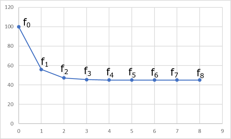
As you can see, this recurrence relation quickly converges to [latex]f_t = 45[/latex] by the time [latex]t = 3[/latex]. That's why the trick works! If we started somewhere else, the graph looks much the same and it converges to 45 anyway.
However, recurrence relations are useful for more than just magic tricks.
Well, since this is a recurrence relation, we want to relate the quantity under consideration, [latex]h_t[/latex] to its value the next year, which is [latex]h_{t+1}[/latex]. So it will look something like
[latex]h_{t+1} = 1.5 h_t + 16[/latex]
but those aren't the right values yet -- just want to have some idea of where this is going.
The first thing we need to encode is the expansion by [latex]1\%[/latex]. We can take [latex]1\%[/latex], or [latex]0.01[/latex] and multiply by [latex]h_t[/latex] like so: [latex]0.01 h_t[/latex]. But the old forest is still there (except for the logging, which we'll worry about in a second), so let's add [latex]h_t[/latex] as well: [latex]0.01 h_t + h_t[/latex]. If we factor out [latex]h_t[/latex], we get \begin{align*}
0.01 h_t + h_t & = h_t(0.01 + 1) \\
& = h_t(1.01) \\
& = 1.01 h_t
\end{align*}
This is the growth by [latex]1\%[/latex]. What about that logging? Well, that's not a percent change, so we'll just subtract the [latex]2000[/latex] to represent the loss of biomass. So our final recurrence relation is-->
[latex]h_{t+1} = 1.01 h_t - 2000[/latex]
Well, let's play with it a bit and see what happens. But before we can do that, we need an initial value [latex]h_0[/latex]. Let's guess something. Since we are losing [latex]2000[/latex] a year, we'll need a much bigger number than [latex]2000[/latex]. Let's just guess that [latex]h_0[/latex] is [latex]50,\!000[/latex] metric tonnes.
Now we can compute several [latex]h_t[/latex] values:
\begin{align*}
h_0 & = 50000 \\
h_1 & = 1.01(50000)-2000 = 48500 \\
h_2 & = 1.01(48500) - 2000 = 46985 \\
h_3 & = 1.01(46985) - 2000 \approx 45500 \\
\end{align*}
We can see that the biomass is going down -- not a good sign for the forest. We can speed these calculations up quite a bit in excel. If you do that, you can see that the forest will be totally gone in by [latex]h_{29}[/latex], in less than thirty years. However, that's not a full answer, since it may depend on how much biomass we start with. Suppose it's a larger forest with [latex]h_0 = 300,\!000[/latex]. Then we see
\begin{align*}
h_0 & = 300000 \\
h_1 & = 1.01(300000)-2000 = 301000 \\
h_2 & = 1.01(301000) - 2000 = 302010 \\
h_3 & = 1.01(302010) - 2000 \approx 303000 \\
\end{align*}
And the forest just grows from there.
Let's see an even more complicated example.
\begin{align*}
f^0_{t+1} & = 5.23 f^3_t + 18.0 f^4_t + 24.55 f^{5+}_t \\
f^1_{t+1} & = 0.277 f^0_t \\
f^2_{t+1} & = 0.3405 f^1_t \\
f^3_{t+1} & = 0.4675 f^2_t \\
f^4_{t+1} & = 0.4675 f^3_t \\
f^{5+}_{t+1} & = 0.4675 f^4_t + 0.4675 f^{5+}_t \\
\end{align*}
Explain what each number in these recurrence relations mean.
My goodness, that's a complicated mess of symbols. But with a little patience, we can figure it out I think.
Let's start with the line [latex]f^1_{t+1} = 0.277 f^0_t[/latex]. We know from the problem statement that [latex]f^0_t[/latex] are the trout of age 0 at year [latex]t[/latex]. The quantity [latex]f^1_{t+1}[/latex] is the amount of one year old trout at year [latex]t+1[/latex]. This equation is relating the number of [latex]0[/latex] year olds with the number of [latex]1[/latex] year olds a year later. What it is saying is [latex]0.277[/latex] times the number of zero year olds gives you the number of one year olds a year later. In other words, this equation is giving a [latex]27.7\%[/latex] survival rate from age zero to age one.
From here, we can now easily decode several other equations. [latex]f^2_{t+1} = 0.3405 f^1_t[/latex] gives a [latex]34.05\%[/latex] survival rate from age one to age two. The similar we find [latex]46.75\%[/latex] survival rate from age two to age three, and the same rate from age three to age four. The equation [latex]f^{5+}_{t+1} = 0.4675 f^4_t + 0.4675 f^{5+}_t[/latex] is a bit more complicated, since trout of age 5+ come from the age 4 trout, but also the age 5+ stay within that category, so there are two ways to get there. Both of these involve a [latex]46.75\%[/latex] survival rate.
Notice these survival rates are pretty low by human standards. However, there is some good news for the species: look at the first equation [latex]f^0_{t+1} = 5.23 f^3_t + 18.0 f^4_t + 24.55 f^{5+}_t[/latex]. What do you make of this? That's right -- these are the new baby trout! As you can see, there are a lot of new babies that help balance the low survival rates we noticed before. In particular, each three year old produces roughly 5 new offspring, each four year old produces on average 18 new offspring, and an average 5+ year old produces almost 25 offspring.
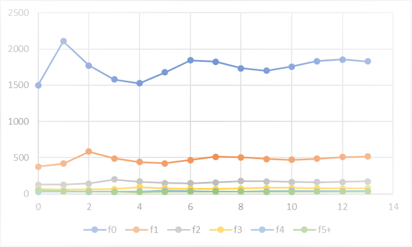
I created this graph in Excel (see the file ``cutthroat-life-cycle.xlsx" for the formulas and data):
And here are just the last four stages to get a better look at these ones:
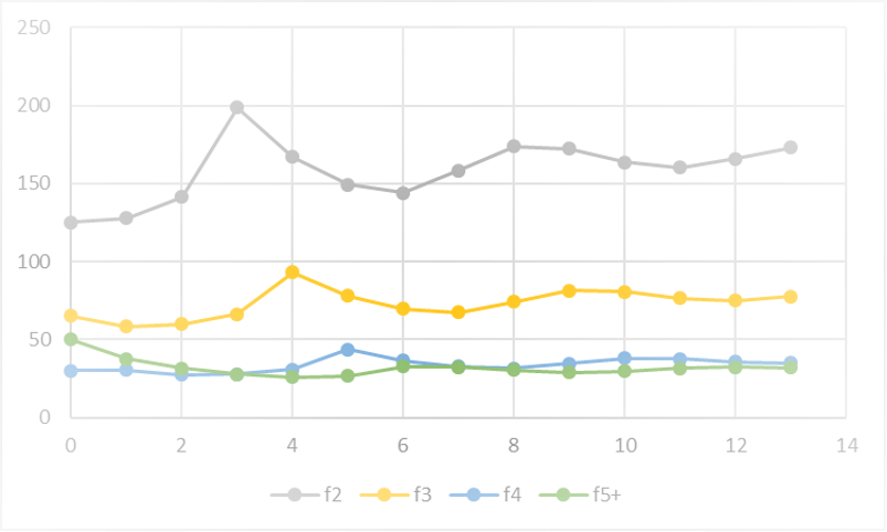
As we can see, the population seems to be fairly stable. One thing that stands out to me is how many age zero and age one fish there are compared to other groups.
