Bio-fluidics

sbeier

4 Bio-fluidics

Even though blood flow operates on micro-scale, not every aspect of microfluidics that has been discussed previously can be transferred directly onto blood. When working with blood flow, the fact that blood is a non-Newtonian fluid as well as the pulsatile flow within an organism have to be taken into account.

4.1 Learning Objectives

Learn how and why blood behaves in certain ways
Discuss the effects of bifurcations, curved and tapered channels
Relate those effects to disease conditions related with blood flow
Understanding the differences in macro- and microfluidics and how it is especially relevant to a range of biological systems.

4.2 Blood rheology

Blood consists of plasma (water, proteins, nutrients, etc), a buffy coat (white blood cells, platelets) and haematocrit (red blood cells). It is a non-Newtonian fluid because its viscosity varies with shear rate, number of haematocrits, temperature and disease conditions. The viscosity increases with increasing shear rate but decreases with increasing haematocrit.

A basic understanding of the rheological or flow characteristics of blood in vivo under normal conditions will help to understand blood flow in abnormal conditions, like obstructed arteries and stenosed valves, prosthetic devices or implants and extracorporeal flow devices. It will also help to reduce trauma to blood and optimise the functionality of blood related devices.

4.3 Casson model

The Casson model incorporates both the yield stress for blood and the shear-thinning viscous properties of blood (Equation 4.1).

It incorporates the yield stress τy, the apparent viscosity η and the shear rate γ̇.

$\sqrt{\tau} = \sqrt{\tau_y} + \sqrt{\mu \dot{\gamma}}$

Under most physiological conditions, the yield stress of blood can be approximated as 0.05 \frac{dyne}{cm^2} = 0.005 \frac{N}{m^2}. Therefore, when a lesser shear stress is applied to blood, blood will not flow, or instead flow as a rigid body.

This phenomenon can be observed when investigating the blood flow profile on a cylindrical channel. In a blood flow developing profile, shear stress at the centreline is zero. Therefore, blood at the centreline needs to flow as a rigid body (Figure 4.1). At the distance ry, the shear stress will exceed the yield stress, and viscous forces take effect.

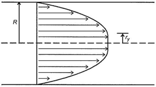
Figure 4.1: Pseudo-parabolic velocity profile of blood ^[2]

Therefore, the blood flow velocity profile has a “blunted” centreline. Blood cells will stream towards the centreline of the blood vessel, because of the microcirculations caused by the non-parabolic flow profile.

4.4 Wave propagation in arterial circulation

Under the progression of pressure/velocity waves, the elasticity of the vessel wall will cause deformation/displacement of the arterial wall. The opening up to the aortic valve, when the heart contracts, creates a pressure wave that travels along the arteries and propels the blood through them, which results in the pulse wave. As it passes through the artery, it causes the arterial wall to dilate.

The velocity with which the pulse wave passes through the artery may be estimated, by accurately measuring both the propagation times between various points of the arterial network and the propagation distance. The temporal resolution with which the pulse wave is captured as it travels along the artery is very important, as this wave travels at a speed, which ranges from several meters per second to tens of meters per second (depending on age, gender, pathology, etc.). Therefore, temporal resolution must be in the order of milliseconds.

Considering a blood vessel that is cylindrical, straight, homogenous and elastic, a pressure pulse at one end of the blood vessel will cause a geometric change in the vessel, which propagates along the tube length at a particular speed. In most in-stances, the wavelength is much larger that the wave amplitude, so the velocity can be seen as one-dimensional. Assuming that the blood velocity is very small, changes in the blood vessel radius is linearly proportional to the blood pressure acting on the vessel wall.

To calculate the blood wave speed c (Equation 4.2), the forces acting on the blood vessel during the pressure pulse p, the conservation of mass, material properties of the vessel wall (e.g. compliance of blood vessel 𝛽), fluid properties and the blood vessel radius ri have to be taken into account.

$c = \sqrt{\frac{r_i}{2\Beta p}}$

If the blood vessel is assumed as purely elastic and relatively thin compared to the diameter and perfectly circular, the wave speed c can be derived from Equation 4.2 to Equation 4.3. Here the elastic modulus E and the thickness of the vessel wall h must be considered.

$c = \sqrt{\frac{Eh}{4pr_i}}$

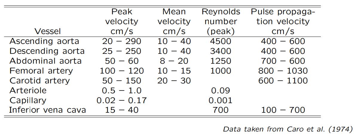
The example of velocity parameters in different arteries and veins can be seen in Table 4.1.

Table 4.1 Velocity parameters in arteries and veins

4.5 Bifurcation

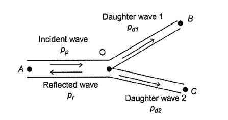
It is very common to have bifurcations in blood vessels. The relationship between parent vessel, daughter vessels and angle of bifurcations (Figure 4.2) can be derived into Equation 4.4 – 4.7 by assuming that the work of supplying tissue with oxygen for each vessel should be minimised.

$r_1 ^3 = r_2 ^3 + r_3 ^3$

$cos \theta = \frac{r_1 ^4 + r_2^4 -r_3 ^4}{2r_1 ^2 r_3 ^2}$

$cos \phi = \frac{r_1^4 - r_2^4 + r_3^4}{2r_1^2 r_3^2}$

$cos(\theta + \phi) = \frac{r_1^4 - r_2^4 - r_3^4}{2r_2^2 r_3^2}$

$Q = Au = \frac{A}{\rho c}p$

$Z = \frac{\rho c}{A}$

$p_p - p_r = p_{d1} + p_{d2}$

$Q_p - Q_r = Q_{d1} + Q_{d2}$

Flow rate can be calculated by multiplying cross-sectional area and flow velocity, where flow velocity can be derived into $\frac{Pressure}{blood \ density \times wave \ speed}$ . Characteristic impedance of blood vessel Z can be different within each vessel. It depends on the blood density, wave speed and cross-sectional area. The pressure difference between incident wave and reflected wave equals to the sum of pressure of daughter branches. Similarly, the flow rate difference between incident wave and reflected wave equals to the sum of flow rate of daughter branches.

Amplitudes of the pressure waveforms can be derived by the prime formula ZQ=p:

$\frac{P_{d1}}{P_p} = \frac{P_{d2}}{P_p} = \frac{2Z_p^{-1}}{Z_p^{-1} + (Z_{d1}^{-1} + Z_{d2}^{-1})}$

There will be a reduction in the pressure pulse through the arterial system, due to energy that is reflected back into the parent branch and subsequently reflected on through the daughter branches.

This analysis can be extended for more complex bifurcating systems and more complex mechanical/physical properties.

4.6 Flow separation

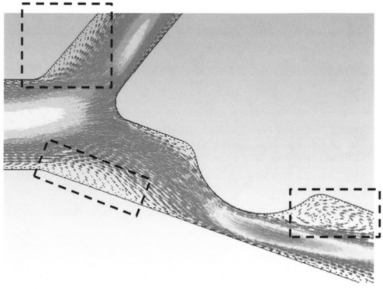
Flow separation is a common occurrence at bifurcations and near the wall when there are rapid geometric changes that expand the cross-sectional area of the blood vessel (Figure 4.4).

Figure 4.4 Flow separation downstream of a bifurcation ^[2]

Flow separation occurs when the flow velocity is relatively fast and cannot expand with the geometry rapidly. Taken into account the corresponding vessel diameter ranging from 800μm to 1.8mm, blood flow rates of 3.0-26 ml/min in arteries and 1.2-4.8 ml/min in veins are obtained.

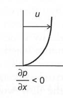
The common way to generate flow separation in biofluid mechanics problems is us-ing the momentum equation (Equation 4.13) if in a pressure-driven viscous flow. Under normal conditions the pressure gradient 𝜕𝑝𝜕𝑥 is negative. As it approaches zero, the flow starts to separate from the wall and as it becomes positive, the flow will completely separate and form a recirculation zone.

$\frac{\delta^2 u}{\deltay^2}\vert _{y=0} = \frac{1}{\mu} \frac{\delta p}{\delta x}$

To maintain the flow regime without recirculation zones, the wall curvature must have the same sign as the pressure gradient (Table 4.2). By quantifying the pressure gradient along the wall, the likelihood for flow separation can be predicted.

Table 4.2 Wall curvature follows the same sign as pressure gradient

Matches the sign of curvature satisfying the momentum equation

Begins to separate from the wall

Completely separate, forming a recirculation zone

4.7 Flow through tapered and curved channels

Tapered blood vessels in biofluidics are assumed to taper in discrete steps, e.g. a continuous taper that reduces the blood vessel radius by half over the entire length. Continuity, momentum conservation and energy conservation can be used to calculate the velocity profile, force, pressure, acceleration, shear stress and other fluid properties in curved and tapered blood vessels.

Curving of the vessel changes the flow profile.

A parabolic profile will be skewed out from the centre of the vessel due to centrifugal forces. This results in a profile with larger velocities closer to the centre of curvature than at the far wall. Vessels gradually narrow (away from the heart) and thus the Reynolds’s number is successively decreased and the flow is stabilised.

4.8 Pulsate flow

Often is assumed that the blood flow is steady, but due to the cardiac cycle, the blood flow is not constant (Figure 4.5).

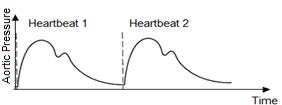
Figure 4.5: Blood flow waveform due to the cardiac cycle

The velocity and pressure waveform are directly related to the contraction of the left ventricle as well as the elastic properties of the blood vessels. Due to the pulsatile nature of the blood velocity and pressure, temporal changes in the fluid parameters should be considered in biofluid mechanics problems.

Here are some parameters that can influence the blood flow:

Pulsating flow, repetition from 1 to 3 beat/sec
Different flow type depends on Reynolds number
Short entrance lengths
Branching
Very complicated flow patterns

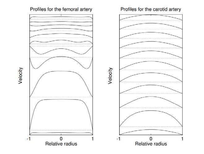
4.9 Womersley numbers

Womersley numbers are related to the pulsatility of the flow. Flows that have regular oscillating time-dependent components (e.g. not steady) are said to have pulsatility. The oscillatory inertia or viscous momentum of fluids α thereby depends in the density ρ, the angular frequency associated with oscillation ω, the characteristic length of the flow L and the dynamic viscosity μ (Equation 4.14).

$\alpha = L(\frac{\omega \rho}{\mu})^{\frac{1}{2}})$

A flow with a low Womersley number is characterised by having essentially no phase difference between the pulsatile pressure waveform that is driving the flow and the pulsatile velocity waveform associated with the flow.

The velocity profiles for different values of Womersley number can be seen in Figure 4.6. The spatial mean velocity is the same for all profiles.

Figure 4.6 Velocity profile under different Womersley number

The influence on velocity profiles for femoral and carotid artery can be seen in Figure 4.7. Profiles at time zero are shown at the bottom of the figure and time is increased towards the top. One whole cardiac cycle is covered and the dotted lines indicate zero velocity.

Figure 4.7 Velocity profiles for femoral and carotid artery

4.10 Pressure waveform

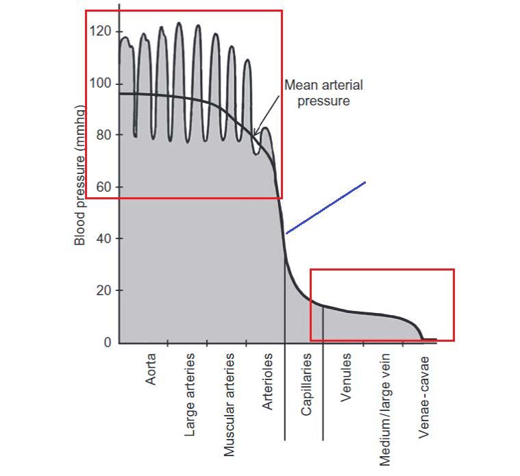
Blood pressure inside of different blood vessels is influenced by not only artery properties but also diastolic pressure and pulse pressure. The mean arterial pressure can be calculated followed by Equation 4.15.

$Mean \ Arterial \ Pressure \ = \ Diastolic \ Pressure + \frac{Pulse \ Pressure}{3}$

The velocity and pressure waveform directly related to the contraction of the left ventricle as well as the elastic properties of the blood vessels (Figure 4.8). Due to the pulsatile nature of the blood velocity and pressure, temporal changes in the fluid parameters must be considered in biofluid mechanics problems. The ways to work around the temporal changes in blood velocity and blood pressure is to consider the discrete steps in time and numerically couples the time steps in Fluid Structure Interaction Modelling.

Figure 4.8 Pressure waveform inside different blood vessels

4.11 Disease conditions

Arteriosclerosis
A disease which arises due to altered fluid dynamic forces, which cause damage to the vascular wall and/or oxidation of lipoproteins which allows plaque to enter the vessel wall and accumulate. This narrows the artery and prevents sufficient blood supply.
Stroke
When the blood vessel leading to the brain becomes blocked with plaque, a stroke may occur. This may result in the blood supply to the brain is interrupted.
High blood pressure
Can increase the risk of damaging vascular walls and cause arteriosclerosis.
Saccular Aneurysm
A bulge in the wall of an artery that is typically caused by a weakening of the muscles within the vascular wall.
Fusiform Aneurysm
It causes artery deformation and rupture. It will cause flow separation and de-crease the compliance of the vessel.

Diseases that affect blood flow, like high blood pressure or arteriosclerosis, can have different influences on the flow inside the vessel, like:

Thickening and stiffening of the arterial walls
Decrease in cross sectional areas of vessels
Causing enhanced shear stress or pressure gradients
Flow can be stagnated around the constriction of the pressure gradient is not large enough to overcome the enhanced resistance to flow
Flow separation from the wall
Decrease mean fluid velocity
Recirculation zone
Reduction in oxygenation
Decrease the compliance of the vessel
Deformation or rupture of the vessel