8 In Vitro Methods
In vitro represents the usage of experimental methodology and procedures for solving fluids engineering systems, This includes full and model scales, large and table top facilities, measurement systems (instrumentation, data acquisition and data reduction), dimensional analysis and similarity and uncertainty analysis. In vitro research is conducted with microorganisms, cells or biological molecules outside of a living organism.
8.1 Learning Objectives
- Describe and analyse different in vitro experimental techniques
- Examine the current state of the art
- Discuss possible future avenues of research in this field
8.2 In vitro experimental techniques
In vitro refers to studies of biological properties that are done in a test tube rather than inside an organism (in vivo). In vitro experimental method can benefit science, technology, research, development and industry areas.
The common in vitro experimental techniques can be divided into either velocimetry and viscometry techniques. Velocimetry techniques measure the velocity of particles in a fluidic system, while viscometry measures the physiological shear stresses applied on cells in fluidic systems.
The process of experimental methods can be summarised into five steps as shown in Figure 8.1.

8.3 Test set-up consideration
The first step in process of experimental methods is the test set-up. It includes facility and condition consideration, model installation, calibration and measurement systems preparation.
Table 8.1 indicates some initial test set-up considerations and instrumentation. First we need to decide the types of measurement. The variable coming from the type of measurement is also an important part in test set-up. After that, the instrumentation should be decided. Then model installation, calibration and measurement systems preparation will be decided based on the goal of the experiment.
Table 8.1 Test set-up initial consideration
| Types of measurement | Variable | Instrumentation | |
| Fluid Properties | Temperature | T | digital thermometer |
| Viscosity | m | viscosimeter | |
| Density | r | hydrometer | |
| Pressure | Surface pressure | Pstat | pressure taps, surface, pressure transducers |
| Stagnation pressure | Pstag | Pitot tubes | |
| Velocity | Flow rate | Q | Venturi-meter, orificemeter, flow nozzle |
| Mean velocity | U, V, W | Pitot tube, hotwire, LDV, PIV etc. | |
| Turbulence quantities |
|
Hotwire, LDV, PIV | |
| Free-surface elevation | z | Point gauge, capacitance wire, servo probe | |
| Force and moment | L, D | Load cell, hydrometric pendulum | |
| Wall shear stress |
|
Preston tube, Stanton gauge, thermal methods (mass and heat transfer probes) | |
![\[ \bar{u' v'} \]](https://oer.pressbooks.pub/app/uploads/quicklatex/quicklatex.com-d2032b0046920d9991bed98bb29df828_l3.png "Rendered by QuickLaTeX.com")
![\[ \tau \]](https://oer.pressbooks.pub/app/uploads/quicklatex/quicklatex.com-7a4f1feafc9bd7a8cd7dc09681ac9dd3_l3.png "Rendered by QuickLaTeX.com")
Three examples of test set-up processes are discussed in the sections below.
8.3.1 Pressure testing in a fluidic system
Instruments in pressure testing in a fluidic system are:
- Manometers: tubes with columns of liquid used to determine pressure differ-ence (P=ρgh). Pitot tubes are frequently used to determine velocities.
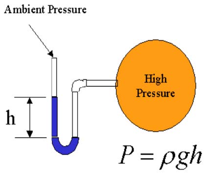
- Pressure transducer: In a transducer, the pressure sensed is converted into mechanical or electrical signal (e.g. diaphragm separating pressure differences and deflects, which changes the capacity C, and then the voltage output E of the circuit).
- Pitot tube: Measuring static and stagnation pressures, using the Bernoulli equation to get flow velocity at the probe.

- Venturi meter: Pressure taps located immediately up- and downstream of the venturi meter’s variable diameter, flow rate is then determined through the Bernoulli and continuity equation.
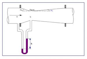
Figure 8.5 Venturi meter
8.3.2 Measuring particles velocity in a fluidic system
8.3.2.1 Particle imaging velocimetry (PIV)
Particle imaging velocimetry is a computer-based technique that tracks reflective particles through a flow chamber. Basic PIV techniques use one camera to obtain flow information, but it is more common to use more than one to collect multiple views to obtain a more complete 3D velocity profile. Using multiple cameras also help re-cording flow patterns because information about the same particles within the flow field is easier to obtain.
The most popular technique for PIV is called particle tracking. One or more cameras image a 3D velocity profile and project it on a 2D plane. Particle tracking often uses fabricated models that depict the geometry of the real flow conditions. Because in most cased the model is scaled up or down from the real scenario, dynamic similarity must be achieved, which was discussed previously.
To collect data with PIV, reflective beads are placed in the fluid. A high-intensity light source (commonly a laser) is focused on the region of interest and a high frame rate camera collects data on particle motion over time (Figure 8.6). By using a computer algorithm, the particle’s velocity can be calculated from the change in position of the particle divided by the frame rate of the camera (Ve-locity = direction × (distance a particle travels/ Δt)). The collection of multiple data sets also makes it possible to obtain mean velocities throughout the flow field.

One problem with particle tracking is that the computer algorithm might not be able to correlate the correct particles in subsequent images. This happens if the particles are either too concentrated or too sparsely within the flow field. If there are too many particles, the algorithm cannot differentiate between individual particles and, if not enough particles are in the fluid, not enough data can be obtained. It is necessary to optimise the particle seeding density in the flow chamber to collect accurate and useful data.
PIV systems are mostly used in biofluid mechanics research to create new designs for cardiovascular implantable devices. Those devices can be tested to determine if they disrupt the flow field and if so, how much it is altered.
8.3.2.1.1 Digital particle imaging velocimetry (DPIV)
Digital particle imaging velocimetry is used to measure the mean velocity of particles in a flow field. Two short laser flashes illuminate the flow area and the illumination is captured by a charge-coupled device (CCD) camera that is connected to a computer. A computer software processes the data of each frame and extracts the velocity vec-tors to create the mean velocity profile of the flow (Figure 8.7).
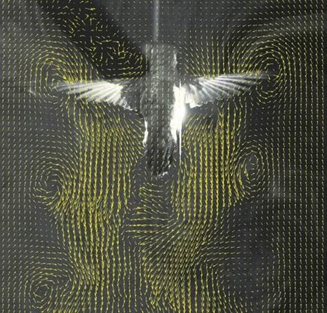
Regular DPIV measures flow fields in two dimensions, but it can be advanced to capture three-dimensional flow field with an additional camera. This complicates the process because more precise timing between laser and camera as well as higher processing power of the computer is necessary.
8.3.2.1.2 Micro particle imaging velocimetry (μPIV)
The measurement of small flow fields isn’t possible with regular PIV technology. To experiment with microfluidic devices, a special technique called micro particle imaging velocimetry is used, where nanoscale fluorescent particles flow through the de-vice. The fluorescent particles are used to remove strong background lighting from the flow. Because of the small scale, the light source and the view field are introduced through the same optics (volume illumination technique).
8.3.2.1.3 Holographic particle imaging velocimetry (HPIV)
HPIV is another PIV technique to obtain a 3D velocity profile. A computer recon-structs an image of the profile after information about the particle location is collected on a hologram. The advantage is that a true 3D flow profile image, instead of one that is projected onto a 2D plane, can be obtained. Instead of using reflective particles and a digital camera, HPIV works with fluorescent particles and an epifluorescent microscope that is linked to a camera. Fluorescent particles have the ad-vantage, that they excite on one particular wavelength of light and emit at a second. Those particles are also smaller than reflective particles and therefore are more useful for studies in microcirculation. The problem is that the fluorescence may over-power small features within the flow field.
8.3.2.2 Laser Doppler Velocimetry (LDV)
Similar to PIV, laser Doppler velocimetry mainly deals with quantifying the microstruc-tures of flows that are subjected to obstacles within the flow field. The advantage of LDV is that the smallest flows surrounding obstructions which may not appear using PIV, can be observed. To measure the fluid velocity, two laser beams intersect at the point of interest. The beams must be monochromatic and coherent to create an inter-ference pattern when intersecting. This pattern occurs within the fluid flow and is cap-tured with a digital camera. As a particle moves through the area of intersection, scattered light will have a different intensity and frequency. This new frequency (ω) is directly related to the fluid velocity, the wavelength and the angle between the laser beams (Equation 8.1).
![\[ \omega = \frac{2v sin(\frac{\theta}{2}}{\lambda} \]](https://oer.pressbooks.pub/app/uploads/quicklatex/quicklatex.com-95cc85eca022dd4bfb43b69e04894cce_l3.png "Rendered by QuickLaTeX.com")
Also similar to PIV, the number of particles within the fluid is important. To many and the computer cannot determine the right velocity; not enough and the data isn’t meaningful.
Dynamic LDV is an improvement over the standard LDV. It measures the total intensity of the scattered light as well as the fringe pattern distortion. This technique can provide a direct measurement of velocities based on time-average values of scatter intensities.
Cells that are suspended in a fluid, e.g. blood cells, experience shear stresses in their environment. To understand the effects of those shear stresses and the relation to fluid flow, a technique is required to expose cells to precise physiological shear stresses. Different kinds of flow chambers are used for that purpose. They can be generally divided into parallel plate-based- and viscometer-based flow chambers.
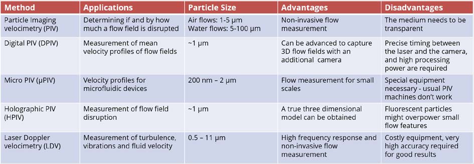
8.3.2.3 Comparison of different velocimetry techniques
The comparison of different velocimetry techniques is summarised in Table 8.2. The choice of instruments for flow velocity experiment can be made based on their applications, particle size, advantages and disadvantages.
Table 8.2 comparison of velocimetry methods
8.3.3 Measuring physiological shear stresses in a fluidic system
Many cells including blood cells are subjected to shear stress in their natural environment. Therefore, there is a need for an accurate experimental technique that can be used to expose cells to precise physiological shear stresses.
There are two types of flow chambers that are typically used in labs:
- Parallel plate-based flow chambers
- Viscometer-based flow chambers
8.3.3.1 Parallel plate-based flow chambers
Parallel plate-based flow chambers use a driving force to push fluid through a rectangular channel. The cells are either seeded in the fluid itself or cultured at the bot-tom surface of the channel. Being at the bottom, the cells will experience a particular shear stress whilst the cells in the fluid are subjected with carrying shear stresses.
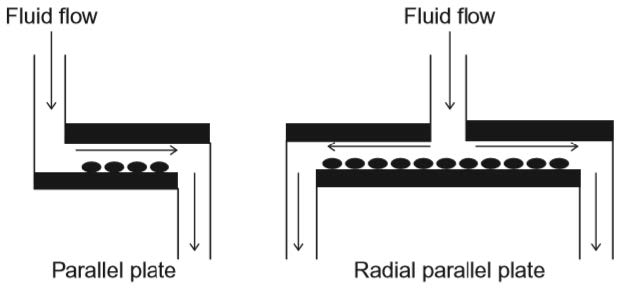
To run successful tests, the flow within the chamber has to be fully developed at the location where the cells are subjected to shear stresses. The shear stress on the walls can be approximated by the Poiseuille equation and is thereby only dependent on the inflow flow rate, the viscosity of the fluid and the channel dimensions. By vary-ing the inflow flow rate different waveforms, like cardiac or respiratory waveforms, can be simulated.
A slightly different version of the parallel plate system is called radial parallel plate flow chamber. Instead of the fluid coming in at one end and exiting on the other, the fluid flows from the centre of the plate and exists in all radial directions (Figure 8.2). The shear stress that is applied is not constant throughout the chamber. It depends on the radial position of the cells. The disadvantage compared to regular parallel plate systems is, that only steady flows (not pulsatilla flows) can be used.
8.3.3.2 Viscometer-based flow chambers
Other viscometry techniques to expose cells to uniform shear stresses are viscometer-based flow chambers. They have no advantage over parallel plate systems but differ in how the experiments are carried out and form a linear velocity profile, instead of a parabolic one, because one of the constraining walls is moving.

Cone-and-plate viscometry is the most common viscometry technique, where a cone is rotated to create the flow profile. To prevent the disruption of the flow profile, the angle between the plate and the cone must be small (0.5˚-1˚). The fluid velocity de-pends on the angular velocity of the cone and the cone angle.
8.4 Data acquisition and reduction
First step of the data acquisition is special considerations. It includes correlate sampling type, sampling frequency, and time with the dynamic content of the signal and the flow nature (laminar or turbulent), consider magnitude of the signal, and identify sources of errors.
The software used in data acquisition is Labview. It is competent in data acquisition, instrument control, analysis and more. It uses graphical programming language for example icons rather than text to built user interfaces with tools and objectives. It uses front panel to control the program.

Data reduction is a step to convert massive raw data into meaningful results, by per-forming statistical analysis (e.g. mean and standard deviation), and/or applying data reduction equations to represents the experiments targeted variable as a function of the measured variables.
8.5 Uncertainty analysis
Uncertainty analysis (UA) is a rigorous methodology for uncertainty assessment using statistical and engineering concepts. It estimates of errors in measurements of individual variables or results. Estimation of uncertainty is usually made at 95% confidence level. It includes two following contents.
Error propagation: Block diagram shows identifications of elemental error sources for individual measurement system or individual measurement vari-ables and their propagation through data reduction equations and to the final experimental results.

- Error sources and uncertainty limits: Error sources comes from bias error β, precision error ε and total error δ=β+ε. Uncertainty limits includes Bias limit B, precision limit P and total uncertainty limit U (U2=B2+P2).
8.6 Data analysis
Data analysis, including but not limited to:
- Curve fitting techniques
- Statistical techniques
- Spectral analysis (Fast Fourier Transform)
- Proper orthogonal decomposition
- Data visualizations
Data analysis compares of the results with bench mark data, CFD, and/or in vivo. It evaluates fluid physics and prepares report.
8.7 Current state of the art in vitro biofluid mechanics research
One of the current major areas of research for velocimetry techniques understands the flow patterns around obstructions or disease conditions using patient specific geometries. The advantage of patient specific models is that the researcher can focus on the effects of flow on one patient and try to predict specific outcomes for another patient.
Many researchers are using these techniques to evaluate existing biofluid implant-able devices in assumed or patient specific geometries. For instance, recent work has evaluated the effects of carotid artery stenosis severity on plaque formations and shear stress levels.
Even though there are some intrinsic limitations to the use of flow chamber-based systems, the information that they provide on basic biology of cells under flow conditions is invaluable. Many groups use these systems to determine the effects of flow conditions on many cellular responses or flow conditions coupled with other risk factors on these same cellular responses. Some areas of research include the genetic profile of a particular cell under shear flow, the proteomic profile of a particular cell under shear flow, how multiple cells interact under shear flow, kinetic reaction rates under flow, disease progression can be monitored and simulated, or new therapeutics can be evaluated under shear flow.
8.8 Possible future avenues of research
One of the major current limitations of in vitro biofluid mechanics research is the availability of models that mimic multiple realistic physiological conditions. For in-stance, most of the techniques use “rigid” wall containers or containing vessels with wall mechanical properties that are drastically different than biological tissue. So, it would be beneficial to simulate the blood vessel walls mechanical properties within their measurements.
As for parallel plate and viscometry techniques, another major hurdle to these experiments is the relevance of the fluid that is perfused throughout the device. In many instances, biofluid mechanics research groups make use of a standard cell culture media or a physiological salt solution as the perfusate, which does not match the physiology well. It may me more relevant to include blood cells within the perfusate, air particles, cytokines, risk factors, hormones, among many other biological relevant chemicals.
Review Questions
Laser doppler velocimetry
Particle image velocimetry
Feedback/Errata