Macrofluidics

sbeier

2 Macrofluidics

2.1 Learning Objectives

Fundamentals of fluid mechanics and fluid dynamics on a macroscopic scale
Important fluid flow and types of fluid flow
Dimensionless numbers
Conservation laws with applications to microfluidics

2.2 Scale

Macro-fluidics refers to fluid problems on a macro-scale, ranging between measurements of millimetres to meters. Fluids behave according to the laws of fluid mechanics and fluid dynamics. Scale is an important consideration, as fluids behave differently on very small scales. In order to minimise the scale of a flow, a certain scale factors “S” must be applied. Each fluid property has a specific scale factor based on their dimension which is indicated by an exponent:

Example: Scaling of a cube

If a cube should be scaled by S=3, the scale factor of each side would be S¹ =3, the scale factor for each surface area would be S² =9 and the volume would have a scale factor of S³ =27.

“Microfluidics is the science and technology of manipulation and controlling fluids, usually in the range of microliters (10^-6 ) to picoliters (10^-12), in networks of channels with lowest dimensions form one (10^-6 ) to hundreds (10^-4 ) micrometers.” ^[10]

Microfluidics deals with the behaviours, precise control and manipulation of fluids that are geometrically constrained to small, typically submillimetre, scale. Typically, “micro” means small volumes, small size, low energy consumption or effects within the micro domain. The science of microfluidics is often used for biological systems i.e. bio flow and applications in health.

2.2.1 Scientific notations

A few common scientific notations with their factor, prefix and symbol are listed in Table 2.1.

Table 2.1: Examples of scientific notations

Factor	Prefix	Symbol
10³	Kilo-	k
10^-1	Deci-	d
10^-2	Centi-	c
10^-3	Milli-	m
10^-6	Micro-	μ
10^-9	Nano-	n
10^-12	Pico-	p

2.2.2 Scaling for forces

Once a certain scale factors S has been applied, the scale factor for different forces can be determined based on their equations. Here are some examples:

The force due to surface tension scales as S¹
The force due to electrostatics with constant field scales as S²
The force due to certain magnetic forces scales as S³
Gravitational forces scale as S⁴

2.3 Intrinsic Fluid Properties

2.3.1 Scaling for forces

Fluids can be divided into different types:

Ideal fluid
Ideal plastic fluid
Real fluid
Incompressible fluid
Compressible fluid
Newtonian fluid
Non-Newtonian fluid

These differences can be summarised into the differences between density and viscosity as listed in Table 2.2.

Table 2.2: Comparison of different types of fluid

Types of Fluid	Density	Viscosity
Ideal fluid	Constant	Zero
Real fluid	Variable	Non-zero
Newtoninan fluid	Constant/Variable	$T = u(\frac{du}{dy}</span><span style="color: #000000">)$
Non-Newtonian fluid	Constant/Variable	$T \neq u(\frac{du}{dy})$
Incompressible fluid	Constant	Non-zero/zero
Compressible fluid	Variable	Non-zero/zero

2.3.2 Density

Density describes the mass of a fluid or solid per unit volume (Equation 2.1) and is defined as $\rho$ .

$\rho = \frac{M}{V} = [\frac{kg}{m^3} = \frac{g}{dm^3}]$

Where M is the mass and V the volume. The density of different fluids is not constant. It depends on the temperature and pressure of the fluid (Table 2.3). Usually density is given at standard atmospheric conditions.

Table 2.3: Examples of different fluid-densities at standard atmospheric conditions

Fluid	Density $[\frac{kg}{m^3}]$	Temperature °C	*Pressure [bar]*
Water	999	20	1.013
Air	1.22	20	1.013
Blood	1060	20	1.013
Ethyl Alcohol	772	20	1.013
Acetone	790	20	1.013
Milke	1035	20	1.013

The density of water at 4 °C ≙ 1000 𝑘𝑔 𝑚³, which is the highest density water can reach, is also used to calculate the specific gravity (SG) of different fluids. To calculate the specific gravity of a fluid, its density is divided by the density of water at 4 °C. Blood for example has a SG = 1.06.

2.3.3 Viscosity

The viscosity is the rate of deformation that a fluid experiences when a shear stress is applied to it, the property of resistance to flow of one layer over another adjacent layer of fluid. Those shear stresses are defined as τ (Equation 2.2). Shear stresses are also directly related to shear forces that are applied to a fluid (Equation 2.3). It can also be interpreted as the internal resistance to changes in motion that will result in deformations.

$shear \ stress = \frac{shear \ force}{area} = \tau = \mu \frac{du}{dy} = [\frac{N}{m^2}]$

$shear \ force = F = \tau A = \mu A \frac{du}{dy} = [N]$

Viscosity is differentiated into dynamic- and kinematic viscosity. Dynamic viscosity µ describes the resistance of a fluid against deformation, as mentioned previously, and its unit is either $[Pa \cdot s = \frac{kg}{m \cdot s}]$ or $\frac{g}{cm\cdot s}$ The kinematic viscosity 𝜐 relates directly to the dynamic viscosity while including the density of the fluid (Equation 2.4). Dynamic viscosity, in general, does not depend on pressure, but kinematic viscosity does.

$v = \frac{\mu}{\rho} = [\frac{m^2}{s}]$

Depending on temperature, the viscosity of fluids changes. Furthermore, as the kinematic viscosity includes the density, it additionally depends on pressure. Generally, with increasing temperature, the viscosity of liquids decreases and the viscosity of gases increases.

2.3.4 Shear dependent fluid behaviour

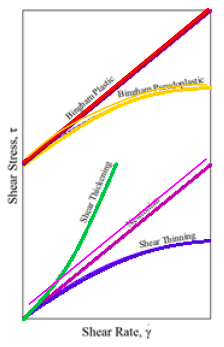
Figure 2.1: Different types of fluids de-pending on shear stress and rate of de-formation

Fluids are divided into different kinds, depending on the relation between applied shear stresses (τ) and the rate of deformation ( $\frac{du}{dy}$ ). The basic differentiation is between Newtonian, Non-Newtonian and Bingham Plastic fluids (Figure 2.1). Newtonian fluids deform proportional to the applied shear stress. Non-Newtonian fluids have no linear relation between shear stress and shear rate. Some Non-Newtonian fluids are called shear thinning fluids or pseudoplastic fluids, because the more the fluid is sheared, the less viscous it becomes. Plastic fluids are those in which the shear thinning effect is extreme. The opposite of shear thinning fluids is shear thickening fluids. These fluids’ viscosity increases with increased shear stresses. In some fluids, a finite stress called the yield stress is required before the fluid begins to flow at all. These fluids are called Bingham Plastic fluids. Bingham Pseudoplastic fluids are Bingham fluids, that have a fluid viscosity which decreases with the increase in shear strain rate.

2.3.5 Compressibility

Alongside the other fluid properties, the compressibility of fluids is often left out, despite its importance. Fluids can be divided into compressible and incompressible (Figure 2.2). The compressibility of a fluid is quantified by the pressure change required to produce a certain increment in either the fluid’s volume or density (Equation 2.5).

$k = \rho \frac{dp}{d\rho}$

Incompressible fluids have a Bulk Modulus k that is mathematically infinite because their density remains close to constant when pressure is applied.

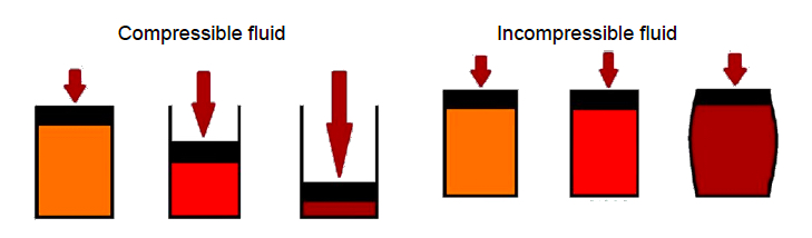
Figure 2.2: Difference between compressible and incompressible fluids

“In general liquids can be treated as incompressible, when the pressure changes are modest. On the other hand, gases are compressible, because according to the ideal gas law, their mass density varies linear with pressure. Despite that, gases can be seen as incompressible for calculations with small pressure changes because the changes in density are also very small.” ^[1]

2.3.5 Surface tension

The surface layer between two different fluids behaves like a stretched membrane due to intermolecular forces. The surface tension (γ) is thereby defined as the force (F) exerted parallel to the surface of the liquid, divided by the length of the line (L) over which the force acts (Equation 2.6). Therefore, the force (F=γL) in surface tension has the scale of S¹.

$\sigma_s = \frac{F}{L}$

2.4 Reynolds numbers

Dimensionless numbers provide a measure of the importance of a phenomenon that plays a role in dictating how this phenomenon occurs. For example, important information regarding the flow domain can be obtained depending on the Reynolds number value. The Reynolds number (Re) provides a measure of which forces dominate changes to a fluid’s velocity and therefore a measure of flow characteristic. It is calculated by dividing the inertial forces by the viscous forces (Equation 2.7). Inertial forces promote turbulent flow, while viscous forces promote laminar flow.

$Re = \frac{inertial \ forces}{viscous \ forces} = \frac{v \cdot D}{v} = \frac{\rho \cdot v \cdot D }{\mu}$

To calculate the Reynolds number the characteristic velocity v, the characteristic diameter D and the dynamic viscosity 𝜇 are taken into account. The characteristic length of the flow through circular equals the pipe’s inner diameter. For a flow through non-circular pipes the Reynolds number is based in the hydraulic diameter D_h (Equation 2.8), which is often derived from the inner area A_c and circumference C and depends on the characteristic shape. The hydraulic diameter of a square duct for example is

$D_h = \frac{4a^2}{4a} = a$

The Reynolds number at which the flow becomes turbulent is called the critical Reynolds number Re_cr. Its value is different for different geometries and flow conditions. For perfect tubes, the critical Reynolds number is 2300. The risk of turbulence thereby increases, with increased velocity, diameter and density, or decreased viscosity. As mentioned previously, the flow characteristic changes depending on the Reynolds number. The distinction is made between laminar, transitional and turbulent flow (Figure 2.3).

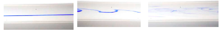
Figure 2.3 Laminar flow, transitional flow and turbulent flow (left to right)

Laminar flow is characterised by highly ordered fluid motion and smooth layers of fluid. The flow of high-viscosity fluids at low velocities is usually laminar. Transitional flow describes a flow that alternates between being laminar and turbulent. Turbulent flow is characterised by highly disordered fluid motion that typically occurs at high velocities.

2.5 Entry Length

The hydrodynamic entry length is usually taken to be the distance from the pipe en-trance to where the wall shear stress (and thus the friction factor) reaches within about 2 percent of the fully developed value.

Hydrodynamic entry length for laminar flow:

$\frac{L_{h, laminar}}{D} \cong 0.06Re$

Hydrodynamic entry length for turbulent flow:

$\frac{L_{h, turbulent}}{D} \cong 0.0693Re^{\frac{1}{4}}$

Hydrodynamic entry length for turbulent flow, an approximation:

$\frac{L_{h, turbulent}}{D} \cong 10$

2.6 Types of fluid flow

2.6.1 Single phase flow & Multiphase flow

Single phase flows are fluid flows that consist of one or multiple fluids in the same phase, e.g. liquid-liquid flows.

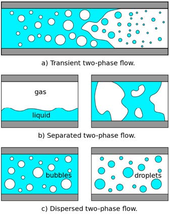
Multiphase flows consist of at least two different fluids in different phases, e.g. gas-liquid flow. Gas-liquid flows can be subdivided into different kinds of two-phase flows (Figure 2.4), like transient, separated or dispersed two phase flow.

Figure 2.4 Different types of two-phase fluid flow

2.6.2 Internal and external flow

The flow inside a pipe or duct if the fluid is completely bounded by solid surfaces is called internal flow.

The flow of an unbounded fluid over a surface such as a plate, a wire or in a channel is called external flow.

2.6.3 Steady & Unsteady flow

The term steady implies no change at a point in time, therefore the velocity, pressure and density of a flow stays the same over any period of time.

The opposite of steady is unsteady, which means that the velocity, pressure or density of a flow varies between different points in time.

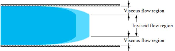
2.6.4 Viscous flow and inviscid regions of flow

Viscous flow describes a type flow in which the frictional effects are significant. Look-ing at a flow through a pipe, viscous flow regions are close to the walls of the pipe.

Inviscid flow regions are flow regions where viscous forces are negligibly small com-pared to inertial or pressure forces. Those flows are mostly of practical interest and happen typically in regions not close to solid surfaces (Figure 2.5).

Figure 2.5: Viscous and inviscid flow regions inside a pipe [12]

2.6.5 Compressible and incompressible flow

In compressible flow, fluid density will change during flow.

In incompressible flow, fluid density will remain constant during flow.

2.6.6 Flow development

Flow development can be divided into the hydrodynamic entrance region and fully developed region (Figure 2.6). Viscous effects due to the shear stress between the fluid particles and pipe wall create a fully developed velocity profile, resulting in the occurrence of fully developed flow. The fluid must travel through a length of a straight pipe to result in a fully developed velocity profile. The velocity of the fluid for a fully developed flow is the velocity at the centre line of the pipe. The velocity of the fluid at pipe walls is theoretically zero. Velocity profiles corresponding to each region can be seen in Figure 2.6.

2.7 Bernoulli equation

The Bernoulli equation is a formula that relates the hydrostatic pressure, the fluid height and the fluid velocity of any two points. The equation can only be used if certain assumptions about the flow are made. The flow has to be steady, incompressible and inviscid. Because of those assumptions the Bernoulli equation can only be used to approximate real flow scenarios.

The equation states that:

Input pressure + input kinetic energy + input potential energy

=

Output pressure + output kinetic energy + output potential energy

The Bernoulli equation can thereby be viewed as a conservation of energy law for a flowing fluid.

$P + \frac{1}{2}\rho v^2 + pgh = const.$

2.8 Macroscopic balances of mass and momentum

2.8.1 Reynolds transport theorem

This theorem relates the time rate of change of each of these properties in a system relative to corresponding changes that occur within and across a control volume. The equation consists of the extensive (i.e. absolute) property B, the intrinsic property (i.e. the amount of that property per unit mass, or, b=B/m) b, the control volume CV and the control surface of that volume CS.

The Reynolds transport theorem can also be reworded as:

Time rate of change of linear momentum in a system =

Time rate of change in linear momentum in the control volume + Net rate of change of linear momentum through control volume surfaces

The change of linear momentum in the system also equals the forces acting on the control volume of the system.

The sum of the forces acting on the control volume can also be rewritten with the body force per unit mass acting on the control volume contents 𝑔⃗ and the stress vector acting on the control ohmic surfaces 𝑡⃗.

2.8.2 Conservation of Mass

Conservation of mass means that the control volume is constant in size and location and the mass of the system is constant. The time rate of change in mass is therefore zero, and any change in mass within this control volume must be equal to the mass of fluid that enters the volume minus the mass that exists.

If the fluid is incompressible, which means the fluid density is constant, the mean velocities multiplied by the cross-section areas result in a constant volume flow rate.

$A_1 \bar V_1 = A_2 \bar V_2 = Q \ (constant \ volume \ flow rate)$

2.8.3 Conservation of Momentum

The conservation of momentum describes the sum of the external forces’ actions on a system. This sum is equal to the time rate of change of the linear momentum of the system.

When the system and control volume are coincident at an instant of time, the forces acting on the system and the forces acting on the control volume are identical:

$\Sigma \overrightarrow F_{sys} = \Sigma \overrightarrow F_{CV}$