Microfluidics

sbeier

3 Microfluidics

Even in small devices and geometries, fluids, especially liquids, can be considered continuous. Hence, well-established continuum approaches for analysing flow can be used as summaries before. The three primary conservation laws that are used to model fluid dynamics are conservation of mass and momentum. Usually at large length scales, the body force F is taken to be gravity. However, because of the square-cube scaling law, where a shape’s volume reduces much faster than its surface area, the effect of gravity in small systems is usually negligible.

3.1 Learning Objectives

Introduce the three primary conservation laws used to model fluid dynamics
Address the capillary effect
Discuss the applications of dimensionless numbers to characterise flow

3.2 Conservation of mass

For a system, the conservation of mass principle states that the net rate of mass flux across the control surface added to the rate of change of mass inside the control volume is zero (Equation 3.1).

$\frac{\delta p}{\delta t} + \nabla(pv) = 0$

3.3 Conservation of momentum

The conservation of momentum principle states that:

Sum of external forces acting in the control volume

=

Net rate of efflux of linear momentum across the control volume + Time rate of change of linear momentum within the control volume

Considering the external forces acting on the control volume, normal and shear stress acting on the control volume under the special case of incompressible, Newtonian fluids, we can get equivalent vector form of the equation (Equation 3.2).

$\p\frac{\delta V}{\delta t} + p(V \cdot \nabla)V = -\nabla p + \eta \nabla ^2 V + pg$

The term a is the “local acceleration of the fluid element”. For a steady flow this term becomes zero. Term b represents the “convective acceleration of the fluid particle”, and it predicts how the flow differs from one location to the next at the same instant of time. The c term is the “pressure acceleration” caused by the “pumping” action. The term d is the “viscous deceleration” term resulting from the fluid’s frictional resistance and term e is the “acceleration caused by gravity”.

Ideal (inviscid) fluid

Considering an ideal, meaning inviscid, fluid, term d can be neglected and the Euler equation (Equation 3.3) forms:

$\p\frac{\delta V}{\delta t} + p(V \cdot \nabla)V = -\nabla p + \eta \nabla ^2 V + pg$

Stokes flow or Creeping flow

In the case of very slow fluid motion, the total acceleration term (term a and b) as well as the acceleration caused by gravity (term e) are zero. The equation then reduces to the equation for Stokes flow or Creeping Flow (Equation 3.4).

$\nabla p = \eta \nabla ^2 V$

When working with very small devices like micro-robots, which among other things are used in the human body to deliver drugs or to scrub out arteries, then Stoke flow should be considered because of the small characteristic length of the system and slow velocity of the fluid, which results in a very low Reynolds number of much smaller than 1 (Re=ρvLμ≪1).

Stoke flow around a sphere is laminar flow. When the sphere changes to different shape, the flow will still be non-turbulent. Since the Stokes flow (which occurs at low Re) is always laminar, independent on the shape of the object.

The drag force FD, on a three-dimensional object of characteristic dimension L mov-ing under Stoke flow conditions at speed V through a fluid with viscosity μ is: FD = constant μVL.

$F_D = 3 \pi \mu VD$

3.4 Capillary Flow

Capillaries are very narrow tubes or confined flow channels.

The capillary effect or action is the ability of a liquid to flow in narrow spaces without the assistance of exter-nal forces. It occurs when the adhesion to the walls is stronger than the cohesive force between the fluid molecules.

Figure 3.1: Example of the capillary effect in water and mercury [13]

The height to which the capillary action will take water in a uniform circular tube is limited by the surface ten-sion. Capillary action occurs when the fluid is at the interface of hydrophobic-hydrophilic surfaces or between hot-cold surfaces, which creates flow. The flow characteristics depend on geometry, wettability, electrowetting and thermowetting (Figure 3.1). The strength of the capillary effect is quantified by the contact angle (θ) defined as the angle that the tangent to the liquid surface makes with the solid surface at the point of contact.

The upward force, tube radius, capillary lift height and capillary pressure can be calculated as below:

This effect is partially responsible for the rise of water to the top of tall trees or to feed oxygen to the brain. When the scale gets smaller, capillary effect increases.

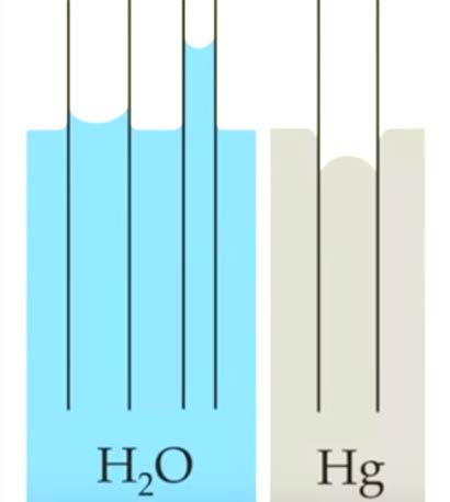
The curved free surface of a liquid in a capillary tube is called meniscus. The curvature of the meniscus depends on the liquid. A hydrophilic liquid like water has a concave meniscus, while hydrophobic liquids like mercury have a convex curvature.

Applications of capillary effect including:

3.5 Poisioulle flow

Newtonian laminar flow inside of a micro-pipe/micro-channel, its volume flow through the pipe per time (flux) can be described as Equation 3.10.

$Q = \frac{V}{t} = \frac{\Delta P \cdot \pi \cdot R^4}{8 \mu L}$

Pressure drop and flow resistance along the micro-pipe/micro-channel can then be described as Equation 3.11 and Equation 3.12.

$\Delta P = \frac{8\mu L Q}{\pi R^4}$

If Newtonian laminar flow flows through a rectangular channel, the volume flow through the pipe per time (flux) can be described depends on the rectangular shape.

For general case,

$Q = \frac{wh^3 \Delta P}{12 \mu L}[1 - 6(\frac{h}{w})\Sigma_{n=0}^\infty \lambda_n^{-5} tanh(\frac{\lambda^n w}{h})$

Where w is the width of rectangular channel and h is the height of the channel.

When h/w<0.7, the equation of flux can be approximated as:

$\frac{12 \mu LQ}{wh^3 \Delta P} = 1 - {6(2^5)}{\pi^5} \frac{h}{w}$

For a channel much wider than the height, h<<w, the velocity profile across the channel is parabolic:

$Q = w \int_h^0 u(y)dy \frac{wh^3 \Delta P}{12 \mu L}$

3.6 Inertial microfluidics

In conventional microfluidic technologies fluid inertia is negligible and flow remains almost within Stokes flow region with very low Reynolds number Re <<1. Inertial microfluidics works in the intermediate Reynolds number range (~1 < Re < ~100) between Stokes and turbulent regimes, and thus still laminar. In this intermediate range, both inertia and fluid viscosity are finite.

Inertial microfluidics has good performance in particle manipulation especially and simple structure, high throughput, and freedom from an external field. Many mechanical effects induced by the inertial effect are difficult to observe in traditional microfluidics, making particle motion analysis in inertial microfluidics more complicated Inertial microfluidics has extensive applications from the ordinary manipulation of particles to biochemical analysis and will play an important role in integrated biochips and biomolecule analysis.

Two key areas of interest in inertial microfluidics are:

Inertial migration: Position of particles migrating through channels with different cross-section shapes called inertial migration.
Secondary flow: In curved channels, central area has higher velocity. Particle through a curved channel flows from centre line to the outward channel because of the inertia causing a radial pressure gradient and the outer fluid is recirculated inwards. Two vortices of opposite directions form in the cross-section of the vertical direction, called “secondary flow“. Characteristics is the dimensionless coefficient De or Dean Number.

3.7 Dean number

The Dean number (De) is a dimensionless group of fluid mechanics, which occurs in the study of flow in curved pipes and channels (Equation 3.16) (Table 3.1).

$De = \frac{\sqrt{\frac{1}{2}(inertial \ forces)(centripetal \ forces)}}{viscous \ forces} = \frac{\frac{1}{2} (pD^2R_c\frac{v^2}{D})(pD^2R_c\frac{v^2}{R_c})}{\mu \frac{v}{D}DR_c} = \frac{\rho D v}{\mu} \sqrt{\frac{D}{2R_c}} = Re \sqrt{\frac{D}{2R_c}}$

Table 3.1: Flow characteristics depending on the Dean number (De)

Dean number		Flow characteristic
< 40-60		Unidirectional flow
40-60 < De < 64-75		Wavy perturbations
> 64-75		Stable pair of Dean vortices
> 75-200		Unstable vortices (twisting, merging, splitting)
> 400		Fully turbulent flow

The Dean flow in particle migration has two main effects:

3.8 Peclet number

Peclet number, Pe, is another dimensionless number representing the ratio of heat transfer by motion of a fluid to heat transfer by thermal conduction. In microsystems, the Reynolds number is too small for turbulent mixing. The mixing in fluids depends on the viscosity and the mass diffusivity D. The higher the diffusivity, the faster fluids will diffuse into each other. The Peclet number measures the magnitude of the advection to the diffusion (Equation 3.6).

$Pe = \frac{U \cdot L}{D}$

If the Peclet number is significantly bigger than 1, the flow rate is high and the diffusion rate low. Peclet >> 1 results in a high diffusion rate. For example, in a T-mixer (a mixer with two inlets and one outlet), where two different fluids are mixed together, the level of mixing depends on the velocity and diffusivity of the fluids. With higher diffusivity or smaller velocity, a smaller mixer is needed for the fluids to completely mix.

3.9 Viscous flow and inviscid regions of flow

In inviscous fluids, the viscosity of the fluid is equal to zero.

The typical Reynolds number range of blood flow in the body varies from 1 in small arterioles to approximately 4000 in the largest artery, the aorta.

The human blood flow spans across a range where viscous forces are dominant to inertial forces being more prominent. Laminar flow is the normal condition for blood flow throughout most of the circulatory system.