7 In Silico
In Silico refers to biological experiments that are performed via computer simulation. This type of research is important because it often takes less time and money than experiments in a laboratory. Of course, this doesn’t make lab-research unnecessary, but can instead help understanding flow relations and create an outlook on the results in vitro or in vivo experiment will deliver. In silico modelling combines the advantages of biological experimentation, without subjecting itself to the ethical considerations nor a lack of control. Complex in silico models are especially valuable when applied to patho-physiological problems, as these methods are able to provide information which cannot be obtained practically or ethically by traditional clinical research methods.
7. Learning Objectives
- Learn how computational fluid dynamics (CFD) works and what it is based on
- Look into dimensionless numbers and how they are created through the Buckingham Pi theorem
- Understand the meaning of dynamic similarity
7.1 Computational Fluid Dynamics (CFD)
7.1.1 Use of CFD
The Navier-Stokes equation, as well as the equations for conservation of mass, momentum and energy can all be simplified by making assumptions and defining boundary and initial conditions. However, in many situations, e.g. unsteady flow, complex body forces or three-dimensional conditions, these equations can’t be easily simplified.
In such cases, computational fluid dynamics (CFD) is a tool which is used to solve coupled Navier-Stokes equations simultaneously by way of conservation equations. CFD employs numerical methods to define flow conditions at discrete points within the volume of interest. As a result, the solution is noncontinuous for the entire flow field.
Example: CFD for Blood Flow
In considering blood flow, CFD is necessary to simulate the flow through arteries or the human aorta. Even though blood can be seen as incompressible within the range of applied pressures, the equations can’t be simplified easily.
This is especially important in areas where the Reynolds number of the flow is around one, which means that neither viscous nor inertial forces dominate the flow. Thus, computational methods are needed to accurately characterise the flow conditions.
7.1.2 Mathematics behind CFD: Conservation laws
The math behind CFD is generally based on the conservation laws which were discussed previously:
- The conservation of mass states, that in an isolated system, mass is neither created nor destroyed by chemical reaction or physical transformations.
- The conservation of momentum means, that in an isolated system with no external forces, the initial total momentum of objects before a collision equals the final total momentum of the objects after the collision (Navier-Stokes-Equations 7.1).
- The third conservation law is the conservation of energy, which states that the total energy of an isolated system remains constant – it is said to be conserved over time.
![\[ \frac{\delta(\rho u)}{\delta t} + \bigtriangledown (\rho u \overrightarrow V) = -\frac{\delta p}{\delta x} + \frac{\delta \tau_{xx}}{\delta x} + \frac{\delta \tau_{yx}}{\delta y} + \frac{\delta \tau_{zx}}{\delta z} + \rho f_x \]](https://oer.pressbooks.pub/app/uploads/quicklatex/quicklatex.com-cb0b681575a603d8c4035998904fff29_l3.png "Rendered by QuickLaTeX.com")
![\[ \frac{\delta(\rho v)}{\delta t} + \bigtriangledown (\rho v \overrightarrow V) = -\frac{\delta p}{\delta y} + \frac{\delta \tau_{xy}}{\delta x} + \frac{\delta \tau_{yy}}{\delta y} + \frac{\delta \tau_{zy}}{\delta z} + \rho f_y \]](https://oer.pressbooks.pub/app/uploads/quicklatex/quicklatex.com-e2abcb596db1ddfdd690f17aa51f2907_l3.png "Rendered by QuickLaTeX.com")
![\[ \frac{\delta(\rho w)}{\delta t} + \bigtriangledown (\rho w \overrightarrow V) = -\frac{\delta p}{\delta z} + \frac{\delta \tau_{xz}}{\delta x} + \frac{\delta \tau_{yz}}{\delta y} + \frac{\delta \tau_{zz}}{\delta z} + \rho f_z \]](https://oer.pressbooks.pub/app/uploads/quicklatex/quicklatex.com-d7f41a4aaf7480624cf1a37539d09a88_l3.png "Rendered by QuickLaTeX.com")
7.1.3 Mathematics behind CFD: Constitutive Equations
In engineering and physics, a constitutive equation is a relation between two physical quantities, especially kinetic quantities as related to kinematic quantities, which is specific to a material, and approximates the response of that material to external stimuli (such as applied fields or forces). For Newtonian fluids, the viscous stresses are proportional to the rates of deformation. The relation between stress and strain is a constitutive equation:
![\[ E = \frac{\sigma}{\epsilon} \]](https://oer.pressbooks.pub/app/uploads/quicklatex/quicklatex.com-cb0d1f7aa7748556a2a9e945451f737a_l3.png "Rendered by QuickLaTeX.com")
7.1.4 CFD workflow process
The process to run a full simulation in CFD can be divided into three steps.
- It begins with pre-processing in which physics, assumptions, boundary conditions, mathematical models, etc. are determined.
- After determination of all variables, the computation process, meaning the CFD solving, starts. Depending on the complexity of the simulation, a high-performance computing (HPC) environment is necessary to finish the simulations in a reasonable amount of time.
- The third step is post-processing where the results are visualised and verified with in vitro and in vivo validation.

In the pre-processing stage, it is important to building an accurate mathematical model. Providing accurate assumptions, boundary conditions and the corresponding mathematical model will lead to a better simulation result.
7.1.4.1 Assumptions
To get more accurate results, we need to use assumptions to simplify if possible. However this is sometimes not possible; in non-stable flow, incompressible flow, complex body forces or three dimensional conditions, then the Navier-Stokes equations cannot be easily simplified. Discretisation is the key for accurate solutions of numerical methods to define the flow conditions.
Blood, interstitial fluid and other biofluids are usually considered incompressible within the range of applied pressures. Furthermore, in arteriole and capillaries, the Reynolds number is much smaller than one; we therefore cannot ignore the inertial terms in fluid mechanics governing equations.
7.1.4.2 Mathematical model and mesh
Using a small element as an example, the possible forces acting on it are caused by direct pressure and shear stress.

The sum of possible forces due to stress in x direction can be written as:
![\[ f_{1x} = (\sigma_{xx} + \frac{\delta \sigma_{xx}}{\delta x} \delta x)\delta y \delta z - \sigma_{xx} \delta y \delta z + (\sigma_{yx} + \frac{\delta \sigma_{yx}}{\delta y} \delta y)\delta x \delta z - \sigma_{yx} \delta x \delta z + (\sigma_{zx} + \frac{\delta \sigma_{zx}}{\delta z} \delta z)\delta x \delta y - \sigma_{zx} \delta x \delta y \]](https://oer.pressbooks.pub/app/uploads/quicklatex/quicklatex.com-e04ff4ba2e2a791eb429ff5160921647_l3.png "Rendered by QuickLaTeX.com")
Equation 7.2 can be rewritten as:
![\[ f_{1x} = (\frac{\delta \sigma_{xx}}{\delta x} + \frac{\delta \sigma_{yx}}{\delta y} + \frac{\delta \sigma_{zx}}{\delta z} \delta x \delta y \delta z \]](https://oer.pressbooks.pub/app/uploads/quicklatex/quicklatex.com-248237d283eabba238fd40be0ad7b6ab_l3.png "Rendered by QuickLaTeX.com")
Similarly, sum of possible forces due to body force in x direction can be written as:
![\[ f_{2x} = \rho B_x \delta_x \delta_y \delta_z \]](https://oer.pressbooks.pub/app/uploads/quicklatex/quicklatex.com-9cbbf4587a72e8ee376d8bdee4de8912_l3.png "Rendered by QuickLaTeX.com")
Based on the equation of motion in x direction F = ma, the equation of motion on this element body is:
![\[ \rho \delta_x \delta_y \delta_z \frac{Du}{Dt} = f_{1x} +f_{2x} = (\frac{\delta \sigma_{xx}}{\delta x} + \frac{\delta \sigma_{yx}}{\delta y} +\frac{\delta \sigma_{zx}}{\delta z} \delta_x \delta_y \delta_z + \rho B_x \delta_x \delta_y \delta_z \]](https://oer.pressbooks.pub/app/uploads/quicklatex/quicklatex.com-f02ce275f826d6ffa295cca382bd89eb_l3.png "Rendered by QuickLaTeX.com")
The Navier Stoke equations in vector notation at x direction can be rewritten from Equation 7.5 to 7.6.
![\[ \rho \frac{D u}{D t} = \frac{\delta \sigma_{xx}}{\delta_x} + \frac{\delta \sigma_{yx}}{\delta_y} + \frac{\delta \sigma_{zx}}{\delta_z} + \rho B_x \]](https://oer.pressbooks.pub/app/uploads/quicklatex/quicklatex.com-d71eeee1a76cc669745a5478f121b786_l3.png "Rendered by QuickLaTeX.com")
![\[ \rho \frac{D u}{D t} = \frac{\delta p}{\delta_x} + \mu \bigtriangledown ^2 u + \frac{1}{3} \mu \frac{\delta}{\delta x} (\bigtriangledown \cdot q) + \rho B_x \]](https://oer.pressbooks.pub/app/uploads/quicklatex/quicklatex.com-e98c26c079c0027363b47ea1fec98163_l3.png "Rendered by QuickLaTeX.com")
The whole body can be divided into thousands of small body elements as shown in Figure 7.3. The division of elements depends on either space discretisation or time discretisation. This thus provides flow conditions at discrete points within the flow field Δ𝑥. Δ𝑥 can be very small, such that you essentially obtain a continuous solution. The whole body will have unknowns from Navier-Stokes Equations like u, v, w. Unknowns like ρ from Continuity Equation, T from Energy Equation and p from The Equation of State will also be considered in the pre-processing phase.

Discretisation directly links to mesh generation in computational simulation. Discretisation breaks down a domain into a mesh, and then replaces derivatives in the governing equation with difference quotients.
Example: Improving mesh accuracy
In computational simulation, different mesh shapes, skewness, aspect ratio and smoothness will directly influence the accuracy of the simulation result.
- In order to achieve high mesh quality, for the same cell count, hexahedral meshes will give more accurate solutions, especially if the grid lines are aligned with the flow.
- The mesh density should be high enough to capture all relevant flow features.
- The mesh adjacent to the wall should be fine enough to resolve the boundary layer flow.
After finalising the mesh, it is important to choose initial and boundary conditions, fluid properties, and the turbulence model. Two commonly used turbulence model are:
- K-ε turbulence model, which is usually used in macrocirculation
- K-ω model, which is usually used at low Reynolds number.
Relevant boundary conditions for different simulation models are further elaborated in ANSYS Fluent.
7.1.5 Applications of CFD in the biomedical area
| Elasticity Problems |
Analysing numerical methods to address the problem of deformation in cerebral structures during treatment planning |
| Air flow in the respiratory system |
Analysis of the pressure distribution of airflow in the tracheobronchial tree |
| Improving heart surgery |
Creating patient-specific software simulation to get a detailed picture of how the blood is flowing, recirculating and moving through the blood vessels. Predictions of influences after intervention are able to be made too. |
| Cardiovascular disease |
Analysing blood patterns in renovascular disease |
7.2 Fluid structure interaction modelling
In some cases, the assumptions that have to be made regarding the physiological aspects of the flow conditions reduce the relevance of a numerical solution. In that instance a different modelling technique called fluid structure interaction (FSI) modelling is used. This modelling technique is especially necessary when a flexible structure with a fluid flowing through it, or it being submerged within a fluid, is simulated.
Example: FSI modelling of the cardiovascular system
The most common example for FSI modelling is of flow though the cardiovascular system. That is because blood vessels are not rigid and show different levels of distensibility depending on the disease condition and the heart pressure pulse. The accurate prediction of those flows therefore needs to take the motion of structure into account. Similar to CFD modelling, the mechanical properties of the vessel must be known or assumptions must be made first to accurately simulate the fluid flow.
An easy method to model solid boundary movement is based on the pressure that the fluid exerts on that boundary at a particular instant in time and space. This method can be used to make a quick approximation if the model parameters are accurate and the flow seems reasonable. To model a more realistic flow, more parameters are used, which makes the equation more complex.
Here a non-linear wave function is coupled to the structure movement. Assuming small body-motion, a uniform pressure throughout the wall and an inviscid and irrotational fluid the wave-function becomes linear (Equation 7.7). This equation can be solved for any fluid property because Ф represents the fluid property of interest, like velocity, pressure, etc.
![\[ \bigtriangledown ^2 \Phi - \frac{\delta^2 \Phi}{\delta t^2} - u[\frac{\delta^2 \Phi}{\delta x^2} +\frac{\delta^2 \Phi}{\delta y^2} + \frac{\delta^2 \Phi}{\delta z^2}] = 0 \]](https://oer.pressbooks.pub/app/uploads/quicklatex/quicklatex.com-40da98eee3fb482de6a0dafd79653ad4_l3.png "Rendered by QuickLaTeX.com")
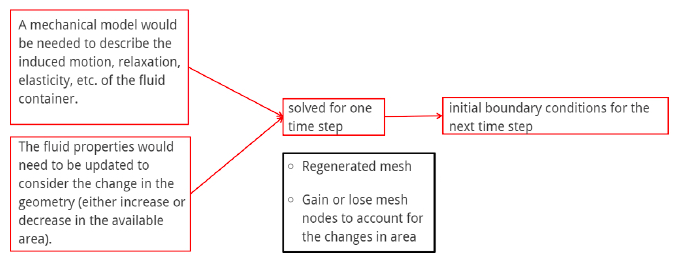
The complexity of FSI is very high: for each time step, the fluid properties must be considered in relation to the motion of the boundary and the changes in boundary position. To solve those models, the changes of the fluid properties due to geometry change must be considered too.
To perform this type of simulation, the parameters that are solved for one time step are used as the boundary conditions for the next time step as shown in Figure 7.4. Results from FSI models in comparison to CFD models for blood flow, show slightly lower flow velocity, because the extensible blood vessel wall would consume kinetic energy.
In addition to blood flow simulation with the blood vessel under disease conditions, FSI models can also be used to investigate interactions of blood cells with the blood vessel wall. These simulations are interesting because they might help understand if the adhesion of white blood cells to endothelial cells under stress conditions can lead to cardiovascular disease conditions.
7.3 Buckingham Pi Theorem
Often, building full-sized prototypes to analyse flow conditions around or inside objects is not an option; the effort to build a realistic model of very large or very small geometries, for example an airplane wing, is just too big and costly. In those cases, the actual flow conditions must be linked to some sort of scaling factor to match the real conditions.
The Buckingham Pi Theorem is a mathematical approach that allows the formation of a relationship between the model and the real scenario. It is a relatively easy approach which is able to obtain a potentially meaningful relationship between all fluid properties of interest.
The Buckingham Pi Theorem states that any grouping of n parameters, they can be arranged into n-m independent dimensionless rations (termed Π parameters):
- It begins by listing all of the dimensional parameters involved in the particular problem (this is equal to n).
- Then the fundamental dimensions for each dimensional parameter are listed and the minimum number of independent dimensions is quantified (equal to m).
- A set of dimensional parameters which include all of the primary dimensions is selected and then solved for a relationship between each of these parameters so that the remaining parameters are dimensionless. [David A. Rubenstein, Wei Yin, Mary D. Frame, 2015, p. 479]
Using the Buckingham Pi Theorem many useful dimensionless numbers can be created (Table 7.1). Some of which have been mentioned in previous chapters:
Table 7.1 Important dimensionless numbers developed using the Buckingham Pi Theorem
| Dimensionless number | Equation | Explanation |
| Reynolds number |
|
Relates inertial to viscous forces and describes them as either laminar or turbulent |
| Strouhal number |
|
Important for pulsatile flows. If St > 1, the fluid moves like a plug, if St < 10-4, the velocity dominates the oscillation. |
| Wormersly number |
|
Relates pulsatility to viscous effects. If α < 1, the flow fully develops, if α > 10, the flow will never fully develop (plug-flow scenario). |
| Cavitation number |
|
Ratio of momentum diffusion to thermal diffusion. It provides a criteria to determine whether the flow delivers or retains its heat. If Pr < 1, the fluid won’t retain its heat very well. |
| Weber number |
|
For flows with a free surface. Relates the inertial forces to the surface tension forces. |
| Capillary number |
|
For flows with a free surface. Relates the viscous forces to the surface tension forces. |
![\[ Re = \frac{\rho v d}{\mu} = \frac{vd}{v} \]](https://oer.pressbooks.pub/app/uploads/quicklatex/quicklatex.com-1288e649205f29a71859ff1273c5e3a9_l3.png "Rendered by QuickLaTeX.com")
![\[ St = \frac{fd}{v} \]](https://oer.pressbooks.pub/app/uploads/quicklatex/quicklatex.com-5b2f42552ce112e95189dd0bea4f8e8e_l3.png "Rendered by QuickLaTeX.com")
![\[ \alpha = d(\frac{\omega}{v})^{\frac{1}{2}} = \sqrt{2 \pi \ Re \ St } \]](https://oer.pressbooks.pub/app/uploads/quicklatex/quicklatex.com-fecefa9e88c8de1f7bafff50b882b170_l3.png "Rendered by QuickLaTeX.com")
![\[ Ca = \frac{p-p_v}{\frac{1}{2} \rho v^2}</td> <td style="width: 33.3333%;height: 14px">Relates local pressure to vapor pressure and kinetic energy. With decreasing numbers, it is more likely for cavitation to arise.</td> </tr> <tr style="height: 14px"> <td style="width: 33.3333%;height: 14px;text-align: center">Prandtl number</td> <td style="width: 33.3333%;height: 14px">\[ Pr = \frac{\mu C_p}{k} \]](https://oer.pressbooks.pub/app/uploads/quicklatex/quicklatex.com-18cd510bbc72facc62375fd7553cf48a_l3.png "Rendered by QuickLaTeX.com")
![\[ We = \frac{\rho V^2 L}{\sigma}\]](https://oer.pressbooks.pub/app/uploads/quicklatex/quicklatex.com-905ff7a943a87846d106c02dd8302dab_l3.png "Rendered by QuickLaTeX.com")
![\[ C = \frac{\mu v}{\sigma}\]](https://oer.pressbooks.pub/app/uploads/quicklatex/quicklatex.com-2e4fc097d00d71f70d75536de9cfa554_l3.png "Rendered by QuickLaTeX.com")
7.4 Dynamic similarity
To model a flow, as many dimensionless numbers as possible between the real flow scenario and the model should be matched. To achieve dynamic similarity, the model must be geometrically and kinetically similar and the forces within the model have to be identical.
Geometrical and kinetic similarity means that the shape and the magnitude of each velocity vector must be related to the real flow scenario by a constant scaling factor. The scaling factors for geometrical and kinetic similarity can differ be-tween the two. To maintain dynamic similarity all of the viscous forces, buoyancy forces, inertial forces, pressure forces and surface tension forces, among others, must be matched. When dynamic similarity is achieved, the flow conditions in the model can be related to the real scenario.
Of course, there are cases where the fabrication of a dynamically similar model might be unreasonable, or the dynamic similarity just cannot be achieved. In those cases, it is important to identify the key properties that should be similar, and the other parameters should be as close as possible. Even though the data won’t be 100% accurate, it is still useful when modelling a real scenario. When analysing the data, the parameters that couldn’t be matched must be accounted for.
7.5 Current state of the art for biofluid mechanics in silico research
In silico biofluid mechanics research consists of many different fields. The two most common fields are:
Example: The evaluation of cardiovascular implantable devices
This first area is a very important tool in designing new devices that minimise damage to blood cells or disruption of the flow field. Originally implanted cardiovascular devices often fail due to damaged induced to blood cells and a disruption to the fluid flow. To prevent this, CFD focuses on identifying the critical geometries within the heart valve structure. Using this technique, the devices can be redesigned even before they are made. This saves saves time and money, because CFD is significantly cheaper than building prototypes for in vitro and in vivo research.
Example: Understanding of the development or flow properties that instigate/propagate cardiovascular diseases.
The second research field mostly focuses on atherosclerosis and aneurysm development. Through in-silico methods, it is possible to make patient specific geometries to predict the onset of the disease or determine how the flow field is impacted around the developing disease
7.6 Possible future avenues of research
In the future, in silico biofluid mechanics research should focus on developing models that are more relevant and incorporate more fundamental processes accurately depict specific pathological events. Some areas that are currently underdeveloped are the incorporation of multiple length scales into the model to depict the flow, cellular deformations, kinetics, etc. These types of models, the initial conditions, assumptions and linking functions can provide a great deal of information to the research community.
Review Questions
Experiments performed outside normal biological contexts, often called "test-tube experiments"
Tested within a living organism
The branch of mechanics that deals with the actions of forces in producing or changing the motion of masses.
Kinematics is a branch of classical mechanics that de-scribes the motion of points, objects and groups of objects without considering the forces that cause them to move
Transforming continuous variables into discrete variables
Feedback/Errata