10 Chapter 10 – Orbital Perturbations

Have you ever wondered why we have to boost the ISS back into its orbit every month or so? After hearing time and time again that the earth is not perfectly spherical, do you wonder what effects this has on orbits? The answer to both of these questions is perturbations. Contrary to how we would prefer orbital mechanics to work, true anomaly is not the only COE that changes over time. To some degree, every COE we have discussed up to this point changes. This chapter will discuss why these perturbations exist and how we track them.

First, let us look back at the big picture. Here we start with a position and velocity of a satellite in Earth’s orbit and predict what its position and velocity will be after a certain amount of time.

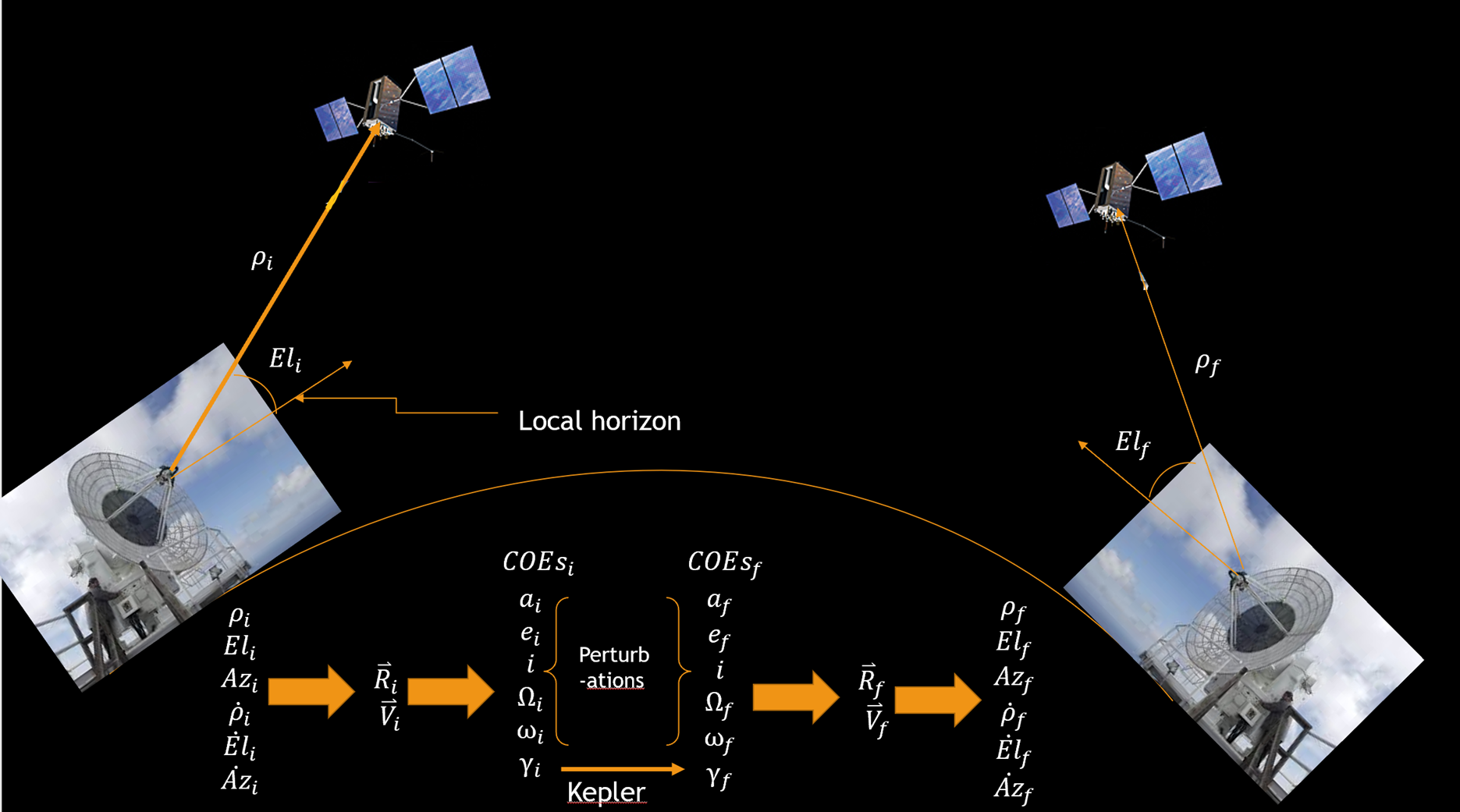
At first glance, it might appear that we have already completed this process using Kepler’s Prediction Problem, but that is in fact not the case. When we initially solved for Kepler’s Problem, we only dealt with an initial and final true anomaly, and we assumed that all other COEs did not change. However, let us look back at our assumptions when we derived the two-body equation of motion and reconsider which ones are actually valid:

1. In order to apply Newton’s Laws in the first place, our coordinate frame must be sufficiently inertial.  Valid
2. The force of Earth’s gravity is the only force acting on the satellite. Not Valid
3. To use Newton’s second Law, we must assume the mass of the satellite (and the earth’s) is not changing. Valid
4. The earth is spherically symmetrical with uniform density. Not Valid
5. The mass of the earth is much greater than the mass of the satellite. Valid

When we made these assumptions, it led our two-body equation of motion (1):

(1)

[latex]\large \ddot{\vec{R}}+\frac{\mu}{R^3} \vec{R}=0[/latex]

However, the equation (2) really looks like (where a_p is the acceleration due to perturbing forces):

(2)

[latex]\large \ddot{\vec{R}}+\frac{\mu}{R^3} \vec{R}=\overrightarrow{a_p}[/latex]

This makes the problem a second order non-linear differential equation. There are two main issues here:

1. Time does not appear, so how is it possible to predict how the COEs change with time?
2. It is a second order non-linear differential equation, so there is no explicit solution.

There are many different ways to solve this problem, with the two main methods being numerical integration and a series solution. We will not delve into how to solve using these methods, but here are the results and the pros and cons from both methods:

Now, considering the general solution, all of our COEs are changing! But why? Let us take a closer look at the second and forth assumptions and why they are not valid.

DRAG

The second assumption we stated was that there are no other forces except gravity acting on the satellite. Unfortunately, this is not true, and the largest contributor is drag. We like to imagine that once we are in space there is nothing. However, if we were to zoom in extraordinarily close to the space a satellite is moving through, then we would see that it is not a perfect vacuum. The atmosphere does get thinner and thinner the higher the altitude, but as long at the satellite is at an altitude less than ~1200 km, then the thin atmosphere will create drag on the satellite.

What is drag? It is a force that works in the opposite direction of motion of an object. This acceleration can be characterized by an equation (3) using area, A, mass, m, velocity (with respect to the atmosphere), V, density of the fluid it is moving through (usually air), ρ, and coefficient of drag, C_D :

(3)

[latex]\large \vec{a}_{\text {Drag }}=-\frac{1}{2} \rho \frac{C_D A}{m} V \vec{V}[/latex]

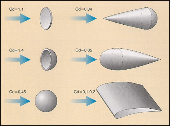
The coefficient of drag varies for different shapes. For example, an object that resists motion and slows down a lot, such as a parachute, has a very high coefficient of drag (~1.5). An object thought to be very aerodynamic, such as a wing (airfoil), will have a very low coefficient of drag (~0.1-0.2). Most satellites tend to have a very high coefficient of drag of around 2. Here are some examples of the coefficient of drag for various shapes in Figure 2:

In astrodynamics, we typically define a new parameter, called the ballistic coefficient, BC, as (4):

(4)

[latex]\large \frac{C_D A}{m}=\frac{1}{B C}[/latex]

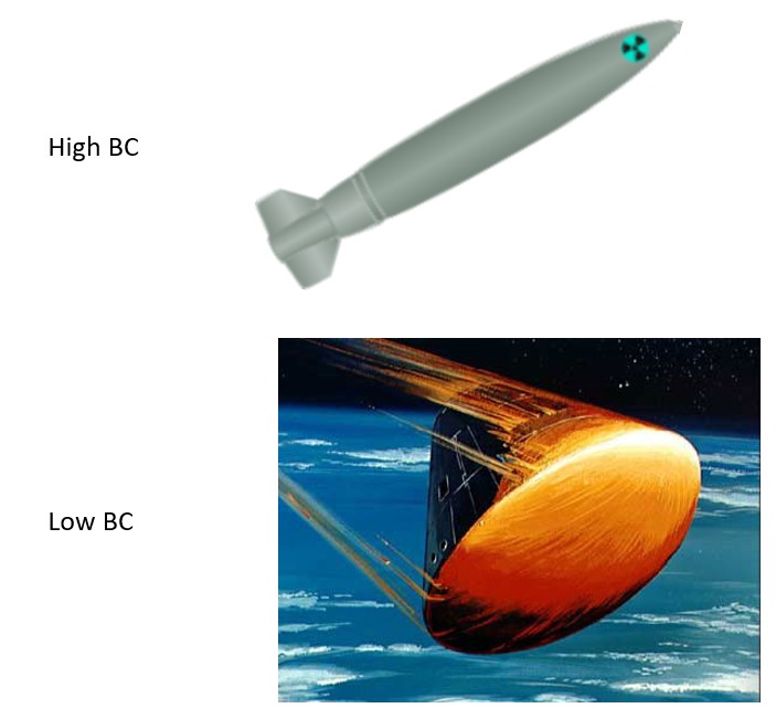
It should be noted that the ballistic coefficient and coefficient of drag are inversely related, so objects with a high coefficient of drag will have a lower ballistic coefficient and vice versa. See Figure 3 below.

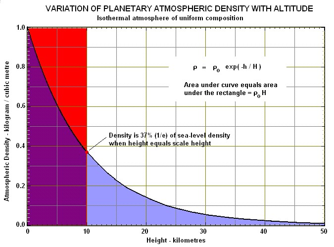
Now that we have defined those coefficients, let us consider the other term that is difficult to model and predict: the density of fluid, which in our case is atmospheric density. The density of the atmosphere gets lower the higher the altitude. Some models define density with an equation (5) using density of the atmosphere at sea level, ρ₀, altitude, h, and scale height, H. This can also be rewritten to use the constant, β.

(5)

[latex]\large \rho=\rho_0 e^{-h / H}=\rho_0 e^{-\beta h}[/latex]

[latex]\large \rho_0=\text { density at sea level }=1.225^{\mathrm{Kg}} / \mathrm{m}^3[/latex]

[latex]\large \beta=\frac{1}{7.315}[/latex]

These equations can be used to plot density versus altitude. Notice this model is only plotted here up to 50 km, much lower than what a satellite would be operating at. See Figure 4 below.

Another modeling method yields the plot below, but once again, note that it is only plotted here up to an altitude of 300 km. See Figure 5 below.

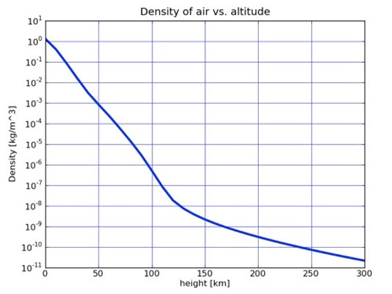
Finally, a third modeling method yields the following plot. Note that this model extends to the altitude we are concerned about for drag effects on satellites in orbit. See Figure 6 below.

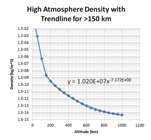
So, now you might be wondering which of these models to use. You will have to decide this for yourself, but for most practical applications– unless given a different model to use– the author recommends the last method.

What effect does this drag have on our orbit? It will actually reduce the size of our orbit after every consecutive pass past perigee. This results in the altitude of perigee remaining approximately constant, while the altitude of apogee gets smaller. See Figure 7 below.

Drag is going to affect specific mechanical energy, ε, semi-major axis, a, and eccentricity, e, making them all smaller. Since a and e are two of our main COEs, then we need to better understand how they are affected. Another value that is going to change is mean motion, n. As the orbit get smaller, the average angular motion gets larger. We can use this value to track the change in semi-major axis, a, and eccentricity, e. We are going to do so by defining these changes over time. How do we do that mathematically? By taking a time derivative, as in Equation 6:

(6)

[latex]\large \frac{d}{d t} n=\dot{n}[/latex]

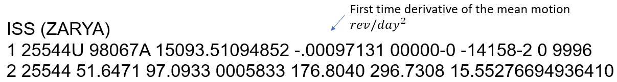
This is great, but where do we get the time derivative of mean motion? It is going to be different for every orbit, but often it is a value that is provided. As you might recall, we previously mentioned the two-line element sets, TLEs, which contain a large amount of information when it comes to an object in orbit. As it happens, the first time derivative of mean motion is one of those values. See Figure 8 below. To see more information, see chapter 6.

Let us begin by using the definition of mean motion and rearranging it into the following form (7):

(7)

[latex]\large n=\sqrt{\frac{\mu}{a^3}}[/latex]

[latex]\large \text { Rearrranging }[/latex]

[latex]\large n^2 a^3=\mu[/latex]

Next, we want to take a time derivative of this equation. Note that both mean motion and semi-major axis are changing with time, so we have to use the product rule to account for both of these derivatives (8):

(8)

[latex]\large \frac{d}{d t}\left(n^2 a^3=\mu\right)[/latex]

[latex]\large 2 n \dot{n} a^3+3 n^2 a^2 \dot{a}=0[/latex]

Then, all we have to do is rearrange for the time derivative of semi-major axis (9):

(9)

[latex]\large \dot{a}=-\frac{2 n \dot{n} a^3}{3 n^2 a^2}[/latex]

Rearranging and Simplifying

Eccentricity is also a value that is decreasing due to drag. It takes a little more creativity to derive this time derivative equation (10). As previously stated, we are going to assume radius of perigee is constant.

(10)

[latex]\large R_p=a(1-e)[/latex]

If this assumption is true, we can use this equation (11) to relate the semi-major axis and eccentricity and solve for the time derivative of eccentricity. Note that since radius of perigee, R_p, is constant, its time derivative is 0. We also have to use the product rule again since both semi-major axis and eccentricity change with time.

(11)

[latex]\large \frac{d}{d t}\left(R_p\right)=\dot{a}(1-e)+a(-\dot{e})[/latex]

Rearranging

[latex]\large -a \dot{e}=-\dot{a}(1-e)[/latex]

Rearranging again

[latex]\large \dot{e}=\frac{-\dot{a}(1-e)}{-a}[/latex]

We can then plug in our previously found equation for the time rate of change of semi-major axis, as in Equation 12:

(12)

[latex]\large \dot{e}=\frac{-\dot{a}(1-e)}{-a}=\frac{-\left(-\frac{2 \dot{n} a}{3 n}\right)(1-e)}{-a}[/latex]

After simplifying, we get the final equation (13) for time rate of change of eccentricity:

(13)

With these values, it may be important to find eccentricity or semi-major axis after a certain amount of time. The future value for any perturbation can be found by knowing the value’s time rate of change using Equation 14:

(14)

[latex]\large x_f=x_i+\dot{x} T O F[/latex]

For more specific equations of eccentricity and semi-major axis, see Equations 15 and 16:

(15)

[latex]\large a_f=a_i+\dot{a} T O F[/latex]

(16)

[latex]\large e_f=e_i+\dot{e} T O F[/latex]

It should be noted that for eccentricity, it is possible to get a negative number. If that happens, that means that perigee and apogee have flipped and the eccentricity is just the absolute value of whatever was calculated.

EXAMPLE 1

Given a semi-major axis, a = 6778 km, eccentricity, e = 0.01, and mean motion time rate of change, [latex]\dot{n}[/latex]=0.001 rev/day², find the semi-major axis after one year.

Try this quiz to test your understanding thus far.

A NON-SPHERICAL EARTH

As mentioned in nearly every elementary school classroom, and contrary to the beliefs of Columbus, the earth is not perfectly spherical. Then what does that have to do with perturbations? Well, much like how drag affects semi-major axis and eccentricity, the earth’s imperfections affect RAAN and argument of perigee of low Earth orbits in the form of a new perturbation called geopotential (commonly called J2 effects). This is contrary to the fourth assumption we stated when deriving the two-body equation of motion: the earth is spherically symmetrical with uniform density. This can be a hinderance in the form of having to define an orbit and how it will change, but there are some orbits that that take advantage of these effects.

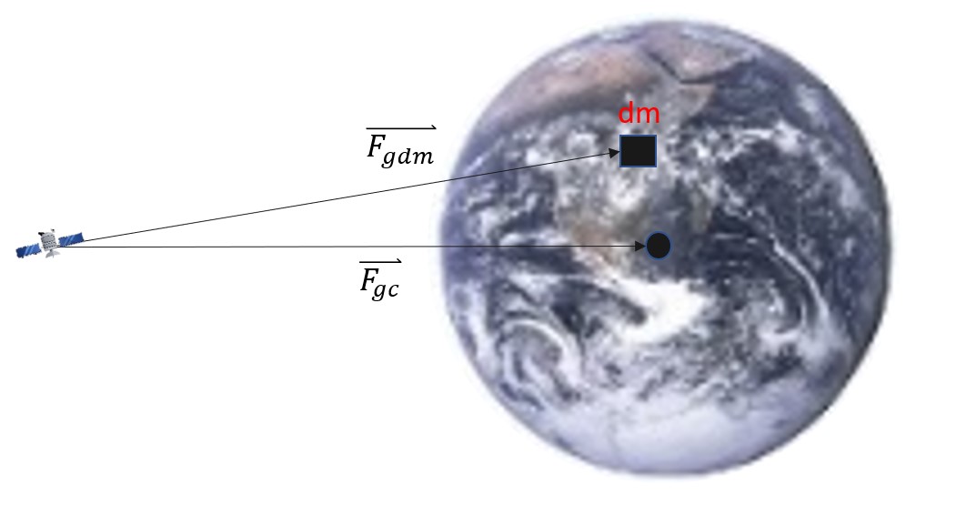
Up to this point, we have treated the earth as a point mass. This means that the conservative force of gravity is pointing to the middle of the earth. Once we no longer treat the earth as a point mass, we have to define another mass (other than the center of the earth), dm, and the gravitational force that the point has on the satellite. We are going to label these as seen in the Figure 9 below:

Because geopotential is a conservative force, we can model it using the simplified potential function with Equation 17:

(17)

[latex]\large \text { Potential: } U=\frac{\mu}{R}[/latex]

In actuality, because the earth is not symmetric, the potential function is usually a function of combinations of harmonic functions. For our purposes, we are going to keep it as a much simpler version. To find the acceleration due to gravity, we take a partial derivative with respect to R. We can also represent this function with the Greek letter del, see Equation 18:

(18)

[latex]\large \vec{a}_g=\nabla=\frac{\partial U}{\partial R} \widehat{R}=-\frac{\mu}{R^2} \hat{R}[/latex]

This function can be modeled with much more detail. The entire potential function takes the form of an infinite sum where coefficients S_LM and C_LM are constants determined from actual satellite data. φ_gc is the geocentric latitude (reference chapter 4 for the difference between geocentric and geodetic) and λ_sat is the longitude. The latitude terms are modeled by Legendre polynomials, the longitudinal terms by Fourier series, and the combined by associated Legendre functions in Equation 19:

(19)

[latex]\large U=\frac{\mu}{R}\left[1+\sum_{L=2}^{\infty} \sum_{M=0}^L\left(\frac{R_e}{R}\right)^L P_{L M} \sin \varphi_{G c}\left[C_{L N} \cos \left(m \lambda_{S A T}\right)+S_{L M} \sin \left(m \lambda_{S A T}\right)\right]\right][/latex]

There are a few different levels of fidelity for geopotential models. We can consider a few of these in order to understand the different effects of these models. The first order model we will consider is when the earth is perfectly symmetric, and where both M and L are equal to 0.

The second model is when only M = 0. Looking at the potential function, this makes all of the sine terms go to 0 and all the cosine terms go to 1. This makes the longitude terms disappear entirely, just leaving the function in terms of latitude. We call this zonal harmonics. Depending on how many terms we consider for L, it can result in more accurate models with the first on the left representing the most significant of these, the J2 effect (equation 20). Right of that is the model given by terms J2 and J3, followed by J2, J3 and J4, and so on. These models each improve their degree of accuracy in representing the earth’s actual shape. See Figure 10 below.

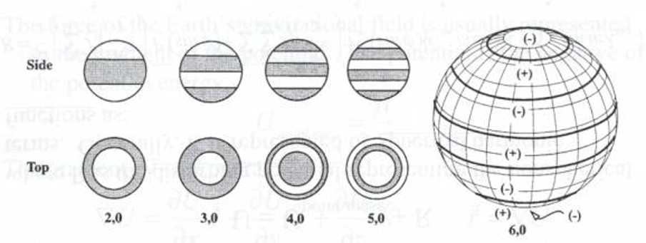
In other words, this model shows different distributions of mass on a latitudinal basis. The 2,0 case can be used to shape a reasonable representation of the largest effect, the Earth’s equatorial bulge. We call this the J2 effect.

The third model sets M=L. This special case makes the geopotential function dependent on only longitude and is called sectoral harmonics. These models take into account extra mass in certain longitudinal directions opposed to the latitudinal ones in model 2. See Figure 11 below.

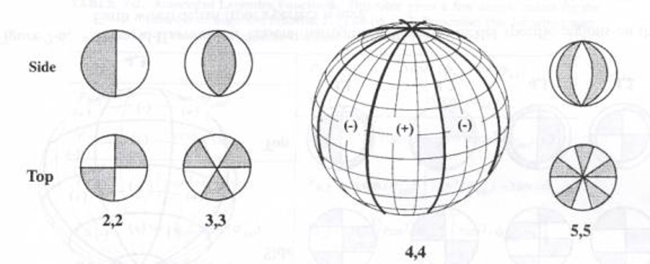
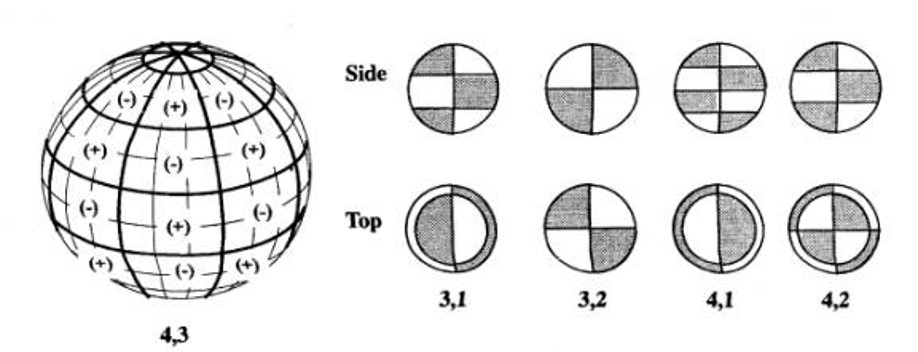
The fourth and last model is the general one where M does not equal L. We call these Tesseral harmonics and the geopotential function becomes a function of both longitude and latitude. These are the most accurate, but the most difficult and complex to solve for and work with. They are generally not needed by basic orbital modeling. See Figure 12 below.

For more on this topic, see Fundamentals of Astrodynamics and Applications by David A. Vallado. Now, let us consider more about the J2 effects.

We have introduced the J2 effect, but what exactly is it? The J2 effect is basically a generalization that the earth bulges at the equator. Think about spinning a ball of dough very rapidly. It is going to become more “squished” where the top and bottom move toward each other causing the size around the “equator” to increase. A very exaggerated image of this can be seen in Figure 13 below. As mentioned before, this can be roughly described by the zonal harmonics with an L value equal to 2. However, what exactly is J2? J2 is a constant that emerges from the geopotential equation that describes this bulge of the earth and is equal to approximately 1082.64×10^-6. Even though this is a small number, it can still affect our RAAN and argument of perigee significantly over time. J2 effects are by far the largest compared to its other J and L effects, about 100 times the effect as its nearest J neighbor, J3 effects. Hence, we often only consider J2 effects when dealing with the geopotential function.

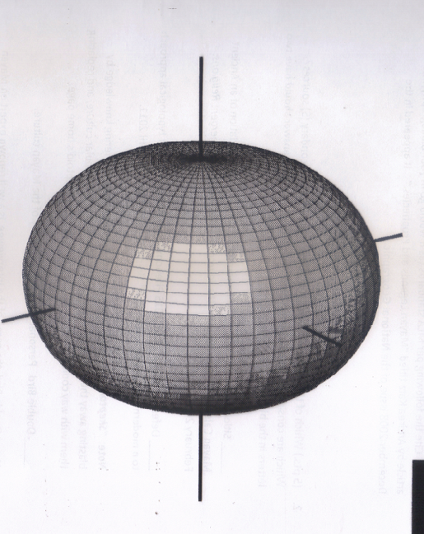
(20)

[latex]\large J_2 \approx 1082.64 \times 10^{-6}[/latex]

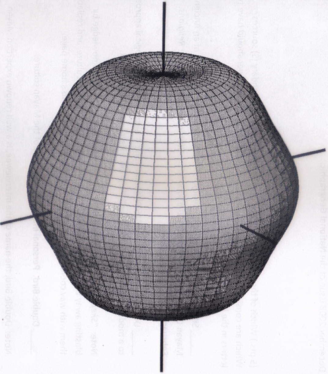
Now let us consider some higher coefficient J effects. Figure 14 is the exaggerated shape of the earth using J3 (Equation 21):

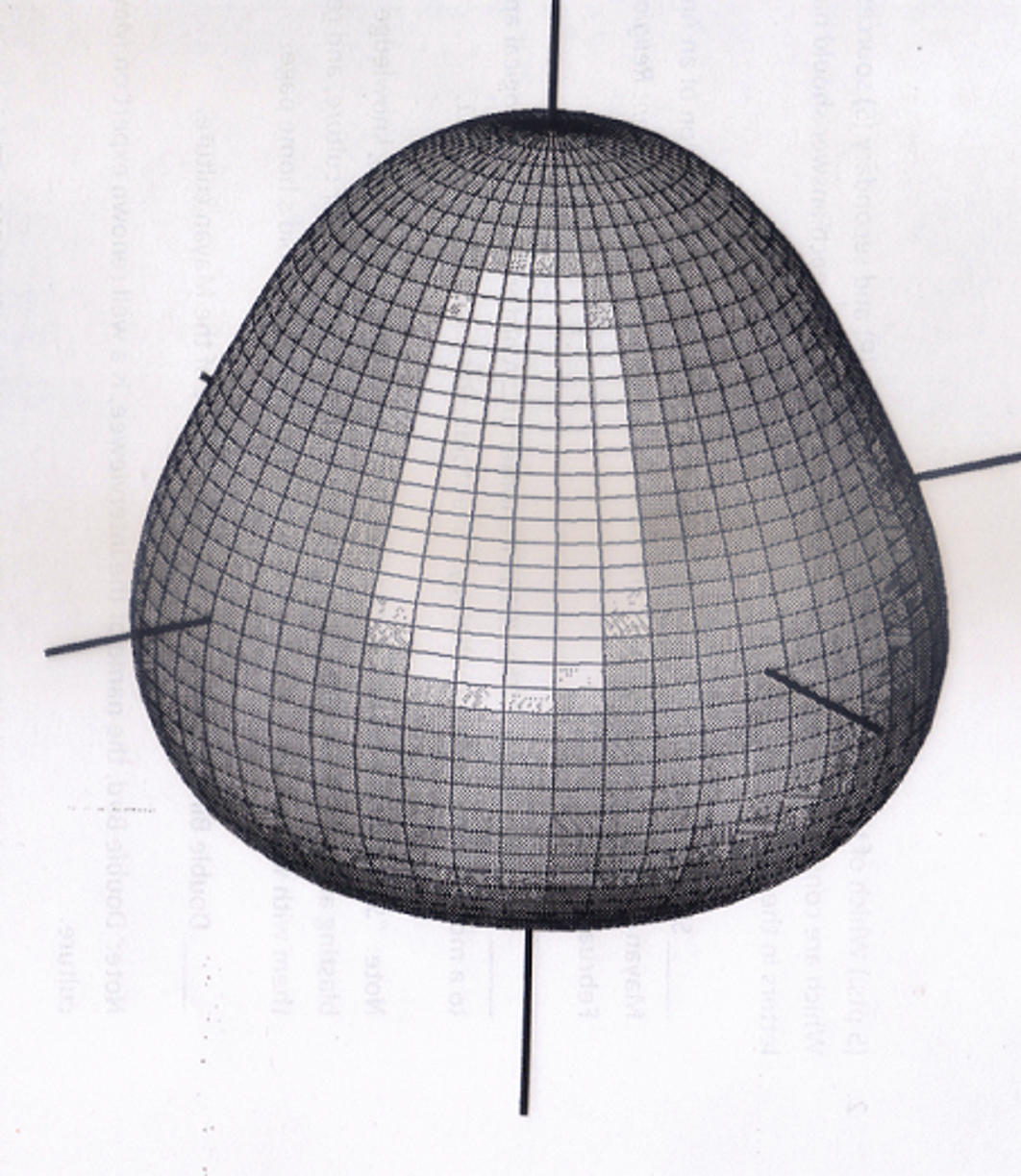
(21)

[latex]\large J_3 \approx-2.532 \times 10^{-6}[/latex]

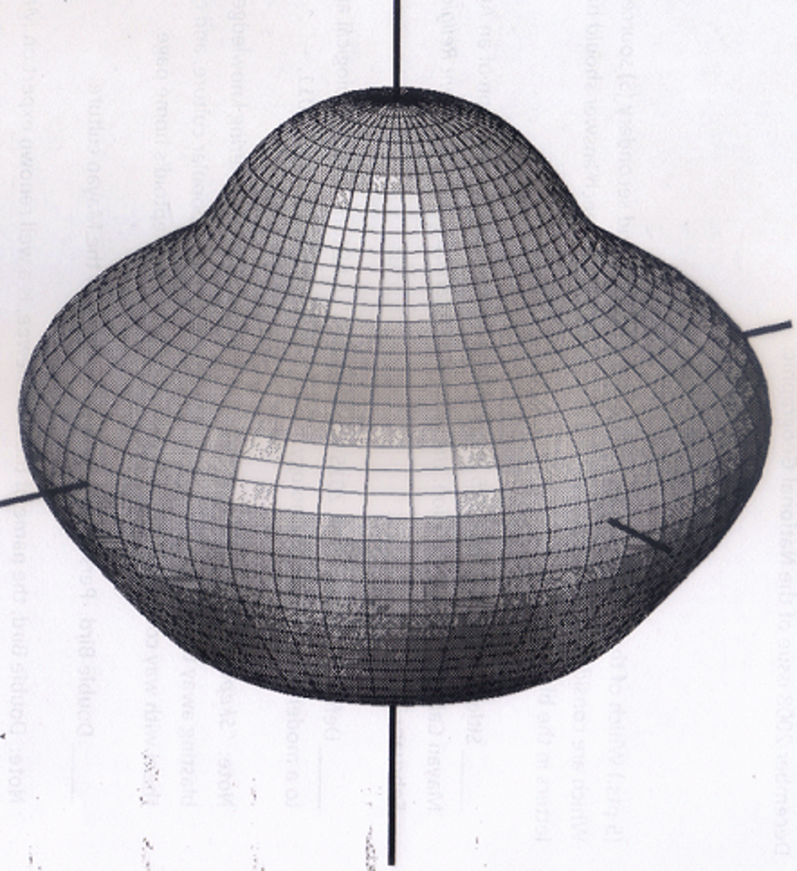
Figure 15 shows J4 effects on Earth (Equation 22):

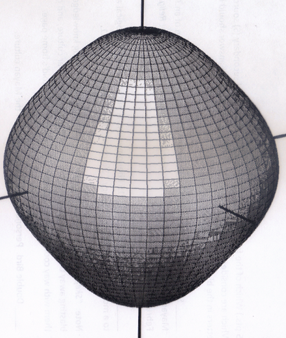
(22)

[latex]\large J_4 \approx-1.611 \times 10^{-6}[/latex]

The J5 (Figure 16) and J6 (Figure 17) effects:

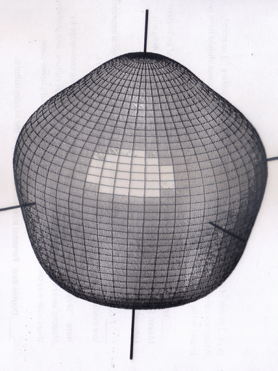
It can be seen that the higher the J effect, the more detail there is to the model. Figure 18 shows a combination of all the J effects from J2 to J6. Wherever bulging is seen is where extra mass appears in the earth model. Again, this is very exaggerated, but it is more accurate than lower terms. It takes about 1,365 coefficients for the model to be accurate to a few meters.

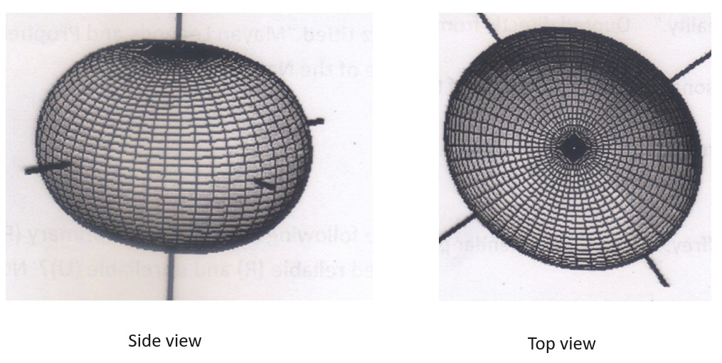
It is also important to note that the above J effect models completely neglected distribution in longitudinal directions. Figure 19 shows the L2 effect and how it does not appear spherical at any angle (even from the top).

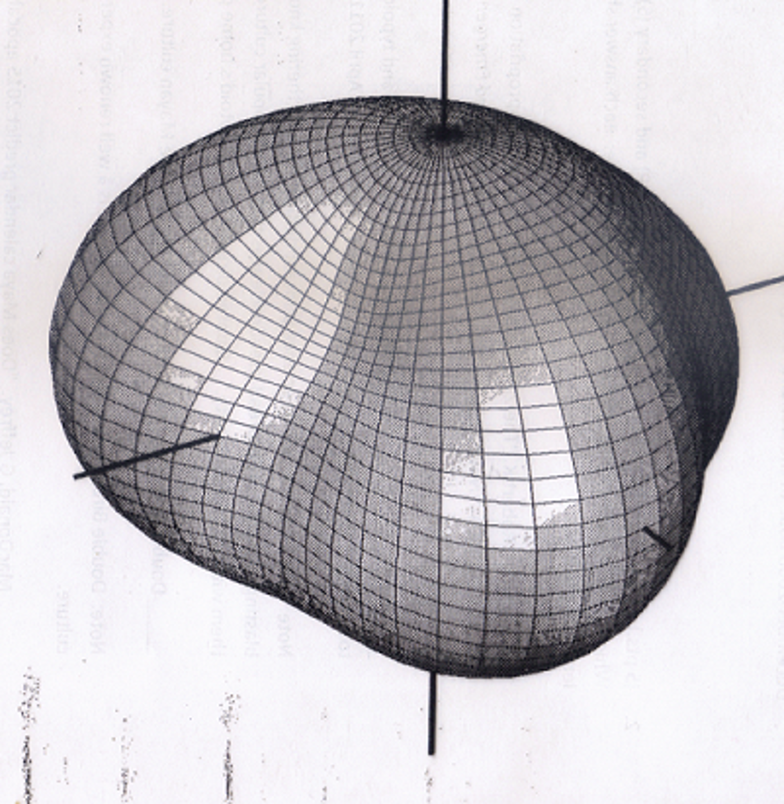
A more exaggerated typical L effect can be seen in Figure 20:

Now, what has this all been leading up to? What effect does this have on our obit? Looking only at the J2 effect, this phenomenon changes both RAAN and argument of perigee. In a low Earth orbit, LEO, both can be affected up to 7-8° per day! In LEO, an orbit can experience different rate of changes at different altitudes and inclinations. A graph can be seen of these changes in Figure 21:

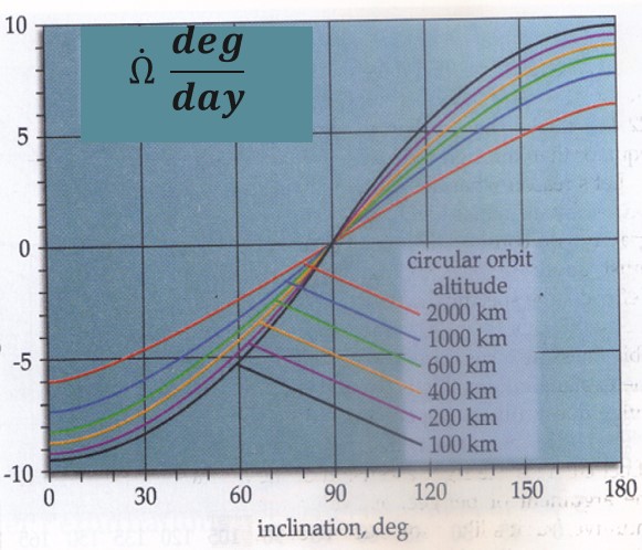
We can also determine this rate of change mathematically using Equation 23:

(23)

[latex]\large \dot{\Omega}_{J 2}=\left[-\frac{3}{2} J_2\left(\frac{R_e}{p_0}\right)^2 \cos i\right] \bar{n}[/latex]

where

[latex]\large p_o=a\left(1-e^2\right)[/latex]

[latex]\large \bar{n}=\left[1+\frac{3}{2} J_2\left(\frac{R_e}{p_0}\right)^2 \sqrt{1-e^2}\left(1-\frac{3}{2} \sin ^2 i\right)\right] \sqrt{\frac{\mu}{a^3}}[/latex]

Argument of perigee is very similar. The effect on argument of perigee depends on inclination and altitude at apogee. This can rotate two different ways depending on inclination. If i < 63.4° OR if i > 116.6°, the major axis will rotate in the direction of the spacecraft’s motion. If 63.4° ≤ i ≤ 116.6°, then it rotates opposite of the satellite’s motion. This can be seen in Figure 22:

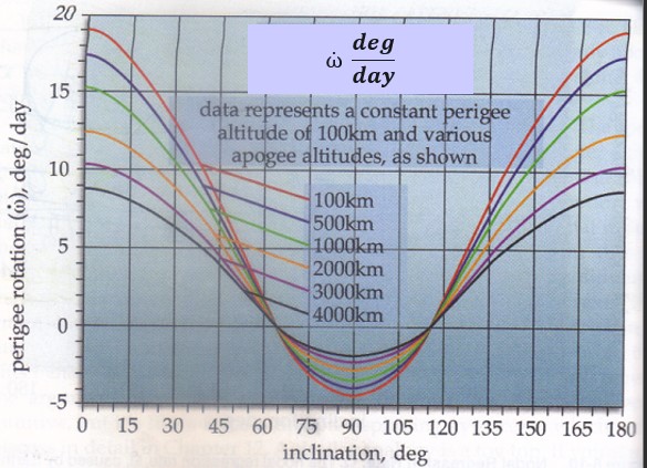
We can also determine this rate of change using Equation 24:

(24)

[latex]\large \dot{\omega}_{J 2}=\left[\frac{3}{2} J_2\left(\frac{R_e}{p_0}\right)^2\left(2-\frac{5}{2} \sin ^2 i\right)\right] \bar{n}[/latex]

where

[latex]\large p_o=a\left(1-e^2\right)[/latex]

[latex]\large \bar{n}=\left[1+\frac{3}{2} J_2\left(\frac{R_e}{p_0}\right)^2 \sqrt{1-e^2}\left(1-\frac{3}{2} \sin ^2 i\right)\right] \sqrt{\frac{\mu}{a^3}}[/latex]

Even though this seems completely detrimental to our orbits, we can use this phenomenon to our advantage. There is a special kind of orbit called a sun-synchronous orbit. It capitalizes on the fact that at about a 98° inclination, depending on altitude, the ascending node moves eastward at approximately 1°/day (more accurately 360°/365 days). This can be seen in Figure 23:

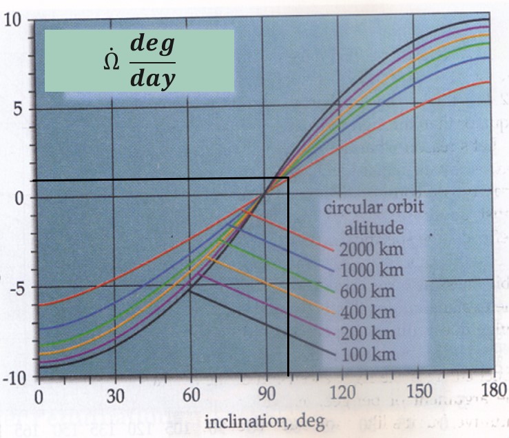
Since the earth also moves around the sun at about 1°/day, the RAAN will process at the same rate the earth rotates around the sun. Thus, the satellite’s orbit will always be at the same sun angle when it passes over specific points on the earth. This can be extraordinarily helpful for imaging satellites, because days and even weeks apart, the images will have the same sun shadows, maintaining great consistency. In other words, you can tell when actual changes happen on the ground versus when the sun’s shadow is moving. This can be used for missions such as reconnaissance, weather, and monitoring the earth’s resources.

Video 1: Sun-synchronous Polar Orbit (Source: EUMETSAT, 2017).

EXAMPLE 2

Given a semi-major axis of a = 6567 km (in LEO) and e = 0, find the inclination of a sun-synchronous orbit. Assume [latex]\tilde{n}=n[/latex]

Another type of orbit that uses geopotential effects to its benefit is a Molniya orbit. Molniya is the Russian word for “fast as lighting.” This 12 hour orbit has a very high eccentricity of 0.7, perigee in the Southern Hemisphere, and an inclination of 63.4°. If we recall, that is the threshold for determining if perigee rotates in the same or opposite direction as the satellite’s motion. Since it is on the cusp of this line, it essentially will not rotate. Video 2 shows a satellite in this orbit in action: 

Video 2: Molniya Visual (Source: Lynn George, 2023).

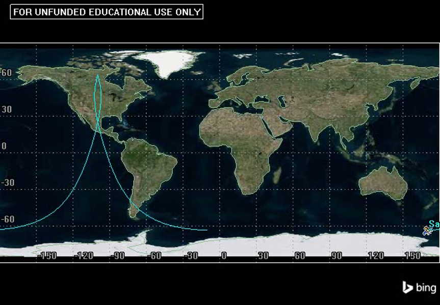
Notice how it stays in the Northern Hemisphere for approximately 11 out of its 12 hour orbit, then it whips quickly through perigee in the Southern Hemisphere, hence the Russian name for “fast as lightning.” Considering the ground track shown below, we can see that the orbit spends much of its time over Russia and the United States. The Russians used this orbit for communication in areas far north (~80° N) where communication satellites in GEO can not be practically used. See Figure 24 below:

EXAMPLE 3

What is the inclination needed for Molniya orbits?

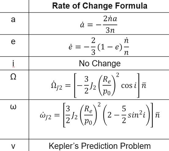
Let us do a quick recap of this chapter. The big picture is that all of our COEs (except inclination, which does change, but is beyond the scope of this text) are all changing. Semi-major axis and eccentricity change due to drag, and RAAN and argument of perigee change due to the J2 effects. The respective equations can be seen in Figure 25:

[latex]\large \mathrm{R}_{\mathrm{e}}=6378.15 \mathrm{~km}[/latex]

[latex]\large J_2 \approx 1082.64 \times 10^{-6}[/latex]

[latex]\large p_o=a\left(1-e^2\right)[/latex]

[latex]\large \bar{n}=\left[1+\frac{3}{2} J_2\left(\frac{R_e}{p_0}\right)^2 \sqrt{1-e^2}\left(1-\frac{3}{2} \sin ^2 i\right)\right] \sqrt{\frac{\mu}{a^3}}[/latex]

Finally, check out this quiz to see how much you understood.

SOLUTIONS TO EXAMPLES:

***EXAMPLE 1 SOLUTION***

Given a semi-major axis of a = 6778 km, eccentricity, e = 0.01, and mean motion time rate of change, [latex]\dot{n}[/latex]=0.001 rev/day², find the semi-major axis after one year.

Solution

The first part of this solution is determining mean motion. Without that, we can not do anything with drag. More importantly, we want this value in rev/day. This is because we are going to look at these values over very large times, so if we had it in rad/s, it would spiral to insane numbers very quickly.

[latex]\large n=\sqrt{\frac{\mu}{a^3}}=\sqrt{\frac{398600.5 \mathrm{~km}^3 / \mathrm{s}^2}{(6778 \mathrm{~km})^3}}=\frac{0.00113 \mathrm{rad}}{s} * \frac{1 \mathrm{rev}}{2 \pi \mathrm{rad}} * \frac{3600 \mathrm{~s}}{\mathrm{hr}} * \frac{24 \mathrm{hr}}{\mathrm{day}}=15.558 \mathrm{rev} / \mathrm{day}[/latex]

We can use this to determine the time rate of change of semi-major axis.

[latex]\large \dot{a}=-\frac{2 \dot{n} a}{3 n}=-\frac{2\left(0.001 \frac{r e v}{d a y^2}\right)(6778 \mathrm{~km})}{3\left(\frac{15.558 \mathrm{rev}}{\text { day }}\right)}=-0.29044 \mathrm{~km} / \mathrm{day}[/latex]

This allows us to determine where semi-major axis will be after a time of flight.

[latex]\large a_f=a_i+\dot{a} T O F=6778 \mathrm{~km}+(-0.29044 \mathrm{~km} / \text { day })\left(1 \text { year } * \frac{365 \text { days }}{\text { year }}\right)[/latex]

We must follow the same process for eccentricity using our pre-determined equation:

[latex]\large \dot{e}=-\frac{2}{3}(1-e) \frac{\dot{n}}{n}==-\frac{2}{3}(1-0.01) \frac{0.001 \frac{r e v}{d a y^2}}{15.558 \frac{r e v}{d a y}}=-4.24219 * 10^{-5} / \mathrm{day}[/latex]

Again, we can use this to determine eccentricity after a year:

[latex]\large e_f=e_i+\dot{e} T O F=0.01+\left(-4.24219 * 10^{-5} / \text { day }\right)\left(1 \text { year } * \frac{365 \text { days }}{\text { year }}\right)=-0.0055[/latex]

Notice that this value is negative. It is not actually a negative eccentricity. This negative just means that apogee and perigee swapped, but the eccentricity is just the absolute value of this calculated value:

***EXAMPLE 2 SOLUTION***

Given a semi-major axis of a = 6567 km (in LEO) and e = 0, find the inclination of a sun-synchronous orbit.

Solution

The most important piece of information of this problem is that the orbit is sun-synchronous. We know that this means the ascending node is traveling eastward at 360°/365 days. This means we already have RAAN rate of change!

[latex]\large \dot{\Omega}_{J 2}=360^{\circ} / 365 \text { days }[/latex]

It is extremely important to watch our units here because every other variable we deal with uses radians and seconds. So we need to convert this value to rad/s.

[latex]\large \dot{\Omega}=\frac{360^{\circ}}{365 \text { days }} \times \frac{\pi}{180^{\circ}} \times \frac{\text { day }}{24 \mathrm{hrs}} \times \frac{\mathrm{hr}}{3600 \mathrm{sec}}=1.992385 \times 10^{-7} \mathrm{rad} / \mathrm{s}[/latex]

Now, let us look at the equation we have:

[latex]\large \dot{\Omega}_{J 2}=\left[-\frac{3}{2} J_2\left(\frac{R_e}{p_0}\right)^2 \cos i\right] \bar{n}[/latex]

If we reorganize to solve for inclination:

[latex]\large i=\cos ^{-1}\left(-\frac{2 \dot{\Omega}_{J 2}}{3 \bar{n} J_2}\left(\frac{p_0}{R_e}\right)^2\right)[/latex]

For this, we need to calculate the semi-latus rectum, which with an inclination of 0 is just equal to a.

[latex]\large p_0=a\left(1-e^2\right)=a=6567 \mathrm{~km}[/latex]

We also need mean motion:

[latex]\large n=\sqrt{\frac{\mu}{a^3}}=1.1868652 \times 10^{-3} \mathrm{rad} / \mathrm{s}[/latex]

With these values, along with the J2 value of 1.08263 𝑥 10−3 and the radius of the earth equal to 6,378 km, inclination can be calculated.

[latex]\large i=\cos ^{-1}\left(-\frac{2\left(1.992385 \times 10^{-7} \mathrm{rad} / \mathrm{s}\right)}{3\left(1.1868652 \times 10^{-3} \mathrm{rad} / \mathrm{s}\right)\left(1.08263 \times 10^{-3}\right)}\left(\frac{6567 \mathrm{~km}}{6378}\right)^2\right)[/latex]

***EXAMPLE 3 SOLUTION***

What is the inclination needed for Molniya orbits?

Solution

Much like example 2, we have one big piece of information. In this problem, we have a Molniya orbit. This kind of orbit is designed to have argument of perigee not change. So in other words:

[latex]\large \dot{\omega}=0[/latex]

We can compare this to the equation we know:

[latex]\large \dot{\omega}_{J 2}=\left[\frac{3}{2} J_2\left(\frac{R_e}{p_0}\right)^2\left(2-\frac{5}{2} \sin ^2 i\right)\right] \bar{n}=0[/latex]

Luckily, many of our terms cancel:

[latex]\large 2-\frac{5}{2} \sin ^2 i=0[/latex]

Solving for inclination, we get:

[latex]\large i=\sin ^{-1}\left(\sqrt{\frac{4}{5}}\right)[/latex]

REFERENCES

Animation of rotating Earth at night.webm. Wikimedia Commons. https://commons.wikimedia.org/wiki/File:Animation_of_Rotating_Earth_at_Night.webm

Aqua Phoenix. (2004). “Segway Human Transporter in Simplified Mechanics.”

Bate, R. R., Mueller, D. D., &amp; White, J. E. (2015). Fundamentals of astrodynamics. Dover Publications.

Colorado Center for Astrodynamic Research (2015). University of Colorado, Boulder.

FSMP (2013). “Nonlinear Wave Equations.”

Hanes, Elizabeth (11 July 2012.) “The Day Skylab Crashed to Earth: Facts About the First U.S. Space Station’s Re-Entry.” History.com.

NASA. (2020, October 5). In depth. NASA. Retrieved March 28, 2023, from In Depth | Hubble Space Telescope – NASA Solar System Exploration

NASA Earth Observatory. (2015) “Three Classes of Orbit.”

Plait, Phil. (13 Nov 2013). “The Last Moments for GOCE.” Bad Astronomy.

Science Blogs. (2010). “Star Trek Jump”

Sellers, J. J., Astore, W. J., Giffen, R. B., &amp; Larson, W. J. Understanding Space An Introduction to Astronautics (3rd ed.). The McGraw-Hill Companies, Inc.

Simple graphic illustration globe showing latitude stock vector (royalty free). Shutterstock. https://www.shutterstock.com/image-vector/simple-graphic-illustration-globe-showing-latitude-13234843

Skeptical Science. (2010). “The Average Temperature Profile of Earth’s Atmosphere.”

SkyJinks. (24 Apr 2015). “What is a Solstice?”

Space Academy (2015).

University of Oregon. Skylab.

Vallado, D. A., & McClain, W. D. (2011)