3 Chapter 3 – The Classical Orbital Elements (COEs)
THE ORBITAL ELEMENTS
In this chapter, we will introduce, describe, and present mathematical equations to find the Classical Orbital Elements, COEs, which are used to locate a satellite in orbit. So far, we have learned to describe where satellites are in orbit by it position, [latex]\vec{R}[/latex] and velocity, [latex]\vec{V}[/latex] vectors. However, these are constantly changing as a satellite moves around its orbit and it is difficult to actually “visualize” where it is.
In this chapter we will reference these vectors to an approximate inertial coordinate frame. We will then learn how these can be used to understand the COEs six parameters that completely describe an orbit and a satellite’s location in it.
1. Its size, a, or semi-major axis, which was introduced in Chapter 2.
2. Its shape, e, or eccentricity, which was also introduced in Chapter 2.
3. Its orbital tilt, or how it is oriented relative to the earth’s equator.
4. Its orientation, or swivel, locating the orbital plane in space.
5. The orientation of the orbit within its orbital plane.
6. The location of the satellite within its orbit, or true anomaly, which was also introduced in Chapter 2
We will first introduce the coordinate frame used for most earth-orbiting satellites, the geocentric equatorial coordinate system, then introduce each of the Classical Orbital Elements relative to that fixed coordinate frame.
THE GEOCENTRIC EQUATORIAL COORDINATE SYSTEM
As we discussed in Chapter 2, when the two-body equation of motion was derived, we found that it was based on Newton’s Second Law. To be valid, Newton’s laws must be based on an inertial, or non-accelerating, coordinate frame.
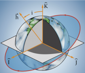
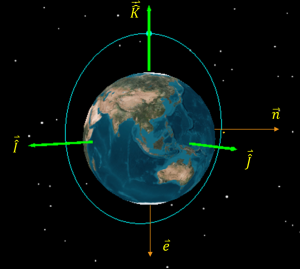
A reference frame is a collection of unit vectors, or vectors with a magnitude of one, at right angles to each other. In the figure below, the black axis would be the coordinate frame, with the unit vectors, [latex]\hat{I}[/latex], [latex]\hat{J}[/latex], and [latex]\hat{K}[/latex] each 90 degrees apart.
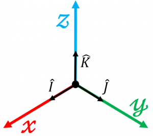
A right-handed coordinate frame is one in which the third axis, [latex]\hat{K}[/latex] in our case, is equal to the cross product of the other two vectors; i.e in Equation (1).
(1)
[latex]\large \hat{I} \times \hat{J} = \hat{K}[/latex]
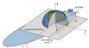
The geocentric-equatorial coordinate system is used for earth-orbiting satellites. It has its origin at the center of the earth. The fundamental plane is the earth’s equatorial plane and the principle axis, [latex]\hat{I}[/latex], points in the vernal equinox direction, [latex]\Upsilon[/latex]. The z-axis, [latex]\hat{K}[/latex], points in the direction of the North Pole. The [latex]\hat{J}[/latex] axis completes the right-handed coordinate frame. The coordinate system is shown in the figure below.
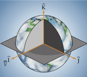
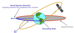
So what is the Vernal Equinox direction [latex]\Upsilon[/latex]? Just as the Greenwich meridian has been arbitrarily chosen as the zero point for measuring longitude on the surface of the Earth, the first point of Aries has been chosen as the zero point in the celestial sphere. It is called the first point of Aries because it was originally in the Zodiac constellation, Aries, as shown in the figure below. This is where the star was located in 150 B.C. when Ptolemy first mapped the constellations. Due to precession of the equinoxes it moved from Aries into Pisces in about 70 B.C., and is now approaching Aquarius (Martin, 2009).
It is also found by drawing a line from the Earth through the Sun on the first day of spring, as shown in the figure below (Kwantus, 2004).
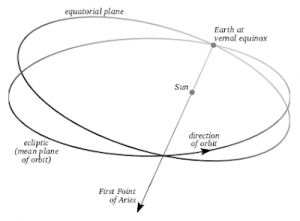
The reason we use this star as our reference is that it is very, very far away (over 160 light-years) from our solar system. As the earth travels around the sun throughout the year, the vernal equinox direction will remain essentially fixed in the same direction, allowing astrodynamics to use this as an inertial coordinate frame.
INTRODUCTION TO THE CLASSICAL ORBITAL ELEMENTS
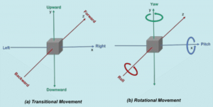
For any physical object we generally need six parameters to describe its location in three-dimensional space. There are three degrees of freedom, x, y, and z as shown in the figure below, and three roll parameters about each axis.
For example, if you are give a position and velocity vector for a spacecraft, it will have six components in the [latex]\hat{I}[/latex], [latex]\hat{J}[/latex], [latex]\hat{K}[/latex] coordinate frame in equations (2) and (3):
(2)
[latex]\large \vec{R} = R_{x} \hat{I}+ R_{y} \hat{J} + R_{z} \hat{K}[/latex]
(3)
[latex]\large \vec{V} = V_{X} \hat{I} + V_{Y} \hat{J} + V_{Z}\hat{K}[/latex]
However, this does not help much in visualizing the spacecraft in its orbit. You cannot tell much about the orbit’s size or shape, nor where the satellite is located in it. Kepler once again came to the rescue and defined a set of six classical orbital elements, sometimes called the Keplerian elements, that were introduced at the beginning of this chapter. We will further investigate these elements one-by-one and see what they tell use about a satellite’s orbit and the satellite’s location in it.
SEMI-MAJOR AXIS, a
The first orbital element we will consider describes the orbit’s size.
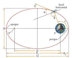
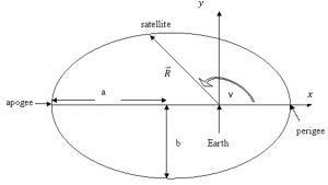
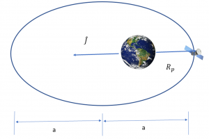
Recall the semi-major axis measures half the distance across the major (long) axis of the orbit, as shown in the figure below. It is a constant parameter in the absence of forces other than gravity since the orbit’s specific mechanical energy does not change.
In Chapter 2, we related the size of the orbit to its specific mechanical energy using the relationship in equation (4):
(4)
[latex]\large \varepsilon = - \frac{\mu}{2a}[/latex]
Where:
[latex]\large \varepsilon[/latex] = specific mechanical energy (km2/s2)
[latex]\large \mu[/latex] = gravitational parameter of central body (km3/s2)
a = semi-major axis (km)
Given a position and velocity vector for a satellite, we can then find specific mechanical energy of the orbit using the relationship in equation (5):
(5)
[latex]\large \large \varepsilon = \frac{V^{2}}{2} - \frac{\mu}{R}[/latex]
Where:
V = magnitude of the velocity vector, [latex]\vec{V}[/latex], in km/s
[latex]\large \mu[/latex] = gravitational parameter of central body (km3/s2)
R = magnitude of the position vector, [latex]\large \vec{R}[/latex], in km
Recall the range of values for each orbit type:
| Orbit type | Semi-major axis value | Comments |
| Circular | a = R >(6378 + 200) km | R radius |
| Elliptical | a such that Rp > 6378 km | Rp = radius of perigee |
| Parabolic | a = [latex]\infty[/latex] | |
| Hyperbolic | a < 0 |
ECCENTRITY, e
Eccentricity describes the shape of an orbit. It is the ratio of the distance between the two foci and the length of the major axis in equation (6).
(6)
[latex]\large e = \frac{c}{a}[/latex]
Thus, it is a unitless quantity. As shown in the figure below, the eccentricity tells you how “out of roundness” the conic section is:
However, this relationship does not provide a convenient way to get the eccentricity from the position and velocity vectors.
The eccentricity of an orbit is also a vector, [latex]\vec{e}[/latex], which points from the center of the earth to perigee and whose magnitude is equal to the eccentricity, e. It is related to the position and velocity vectors using one of two equations, which are equivalent in Equation 7:
(7)
[latex]\large \vec{e} = \frac{1}{\mu}[(V^{2} - \frac{\mu}{R})\vec{R} - (\vec{R} \cdot \vec{V})\vec{V}][/latex]
Or use Equation 8:
(8)
[latex]\large \vec{e} = \frac{1}{\mu}(\vec{V} \times \vec{h}) - \frac{\vec{R}}{\left| \vec{R} \right|}[/latex]
Where:
V = magnitude of the velocity vector, [latex]\large \vec{V}[/latex], in km/s
[latex]\large \mu[/latex] = gravitational parameter of central body in km3/s2
R = magnitude of the position vector, [latex]\large \vec{R}[/latex], in km
[latex]\large \vec{h} = \vec{R} \times \vec {V}[/latex]= specific angular momentum vector in km2/s
The eccentricity is then the magnitude of the vector, or in equation (9)
(9)
[latex]\large e = \left| \vec{e} \right|[/latex]
Alternately, if the Radius of Perigee and semi-major axis, a, are known, you can also find the magnitude of the eccentricity vector using the relationship in equation (10):
(10)
[latex]\large R_{p} = a(1-e)[/latex]
Or if Radius of Apogee and semi-major axis, a, are known, you can find the magnitude of the eccentricity vector using the relationship in equation (11):
(11)
[latex]\large R_{a} = a(1+e)[/latex]
Recall the range of values for each orbit type:
| Orbit Type | Eccentricity Value(s) |
| Circular | e = 0 |
| Elliptical | 0 < e < 1 |
| Parabolic | e = 1 |
| Hyperbolic | e > 1 |
INCLINATION, i
The inclination indicates the tilt of an orbit. It is the angle measured between the [latex]\widehat{K}[/latex] axis and the angular momentum vector, [latex]\vec{h}[/latex], as shown in the Figure 9:
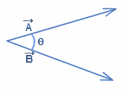
You might be wondering why the angle between the equatorial plane and the orbital plane is not used to describe inclination. Recall from the mathematics review in Chapter 2 that the angle between two vectors [latex]\vec{A}[/latex] and [latex]\vec{B}[/latex] is given by equation (12):
(12)
[latex]\large \cos\theta = \frac{\vec{A} \cdot \vec{B}}{AB}[/latex]
Thus this provides a convenient way to measure the inclination as it is the angle between the two known vectors. The angular moment vector, [latex]\vec{h}[/latex] is given by (13):
(13)
[latex]\large \vec{h} = \vec{R} \times \vec{V}[/latex]
The [latex]\hat{K}[/latex] vector is the unit vector that points from the center of the earth to the north pole, and it is given by [latex]\hat{K} = 0 \hat{I} + 0\hat{J} + 1\hat{K}[/latex]. Hence, the inclination is given by equations (14) and (15):
(14)
[latex]\large cos i = \frac{\vec{h} \cdot \hat{K}}{hK}[/latex]
Since,
(15)
[latex]\large \vec{h} \cdot \hat{K} = h_{I}(0) + h_{J}(0) + h_{k}(1)[/latex]
And K is the magnitude of the [latex]\hat{K}[/latex] vector, or 1, so this expression becomes in equation (16):
(16)
[latex]\large i = \cos^{-1}(\frac{h_{k}}{h})[/latex]
Where:
hk = the kth component of the angular momentum vector, [latex]\large \vec{h}[/latex]
h = the magnitude of the angular momentum vector, [latex]\large \vec{h}[/latex]
The inclination, i, only takes values between 0° and 180°. An explanation of the types of orbits is found in the figure below:
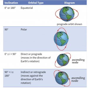
An orbit with an inclination of 0° is called an equatorial orbit because satellites in these orbits travel around the earth’s equator. A Satellite at a geostationary altitude, as calculated in example 2 in Chapter 2, is in an equatorial orbit. This allows it to remain above the same spot on the earth as its eastward velocity is approximately equal to the the velocity of the ground directly beneath it. An orbit with an inclination of 180° could theoretically be used, but it would be travelling in the opposite direction of the earth’s rotation and would be highly inefficient to launch into. A satellite in a polar orbit has an inclination of 90° and hence travels over the north and south geographical poles. This type of orbit allows for maximum viewing of all of the latitudes of the earth.
Satellites can also be categorized as prograde or retrograde. Prograde orbits have inclinations between 0° and 90° and travel in the direction of the earth’s rotation. These are, by far, the most prevalent types of orbits. They are more efficient to launch into because they already have the benefit of the earth’s rotation at the launch site to give the satellite an eastward boost. Retrograde orbits have inclinations greater than 90°. Retrograde orbits with greater than about 110° inclinations are rare as satellite in them travel against the earth’s rotation. There is, however, a well-used orbital inclination at about 98° to 100°, called a sun-synchronous orbit. We will learn later how sun-synchronous orbits are designed and how they are very valuable for earth-observations.
Inclination applies to all orbit types and conic sections. Here is a summary of what we know so far about inclinations:
| Inclination
0 |
Type
Equatorial |
Comments Travels above Earth’s equator If at geo altitude, is geostationary
|
| 180 | Equatorial | Not normally used |
| 90 | Polar | Covers all latitudes
|
| 0 – 90 | Prograde | Satellite travels in the same direction the earth’s rotates
|
| 90 – 180 | Retrograde | Satellite travels in the opposite direction the earth’s rotates
Seldom use orbital inclinations greater than 110 degrees |
RIGHT ASCENSION OF ASCENDING NODE, RAAN, [latex]\Omega[/latex]
The RAAN indicates the swivel or orientation of an orbit. It is the angle measured between the [latex]\hat{I}[/latex] axis and the ascending node vector, or the vector pointing to the location where the satellite passes from the southern to northern hemisphere. First, though, we must define the ascending node vector, [latex]\vec{n}[/latex], sometimes called the line of nodes, as shown in the figure below in equation (17):
(17)
[latex]\large \vec{n} = \hat{K} \times \vec{h}[/latex]
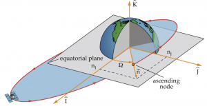
The ascending node vector lies along the intersection of two planes – the orbital plane and the equatorial plane.
RAAN, or [latex]\Omega[/latex], is then the angle measured from the vernal equinox direction, [latex]\hat{I}[/latex], to the ascending node vector, [latex]\vec{n}[/latex]. Hence, RAAN is given by equation (18):
(18)
[latex]\large \cos\Omega = \frac{\hat{I} \cdot \vec{n}}{In}[/latex]
And since the [latex]\hat{I}[/latex] vector is the unit vector that points from the center of the earth to the vernal equinox, hence is give by [latex]\hat{I} = 1\hat{I} + 0\hat{J} + 0\hat{K}[/latex]. Hence, RAAN is given by equation (19):
(19)
[latex]\large \Omega = \cos^{-1}(\frac{n_{i}}{n})[/latex]
Where:
ni = the ith component of the ascending node vector, [latex]\large \vec{n}[/latex]
n = the magnitude of the ascending node vector, [latex]\large \vec{n}[/latex]
RAAN can take any value between 0° and 360° so a half plane check is needed. As can be seen in the figure above, if the jth component of the ascending node vector is negative, then RAAN is in the second half plane. This can be written mathematically as in equation (20):
(20)
If nj < 0 then 180 < [latex]\large \Omega[/latex] < 360 degrees.
As described in the Math review section, remember that for a cosine term, to find the angle in the second half plane, use 360° minus the angle in the first half plane, or in equation (21):
(21)
[latex]\large\Omega[/latex] second half plane = 360 degrees – [latex]\large\Omega[/latex] first half plane
If the ascending node vector points along the vernal equinox direction, then [latex]\Omega[/latex] = 0.The RAAN in the figure shown above is about 45°. In the figure below, it is about 90° and in the second figure below, it is about 270°. Our next COE will be referenced from the ascending node vector.
Note [latex]\Omega[/latex] is not defined if there is no ascending node, in other words if the orbit is equatorial with an inclination of 0° or 180°.
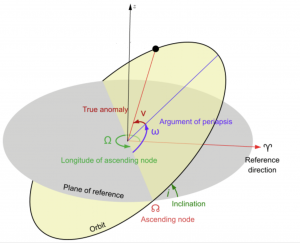
ARGUMENT OF PERIGEE, [latex]\omega[/latex]
The argument of perigee, [latex]\omega[/latex] indicates theorientation of the orbit, or where its perigee is located. It is the angle measured between the ascending node vector, [latex]\vec{n}[/latex], and the location of perigee, at which the eccentricity vector, [latex]\vec{e}[/latex], points.
Hence, argument of perigee is given by equations (22) and (23):
(22)
[latex]\large \large \cos\omega = \frac{\vec{n} \cdot \vec{e}}{ne}[/latex]
Or
(23)
[latex]\large \large \omega = \cos^{-1} (\frac{\vec{n} \cdot \vec{e}}{ne})[/latex]
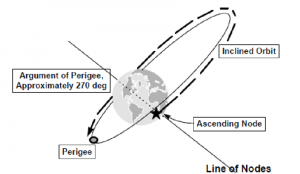
Argument of perigee can take any value between 0° and 360° so a half plane check is needed. As can be seen in the figure above, if the kth component of the eccentricity vector is negative, then argument of perigee is in the second half plane. This can be written mathematically as in equation (24):
(24)
If ek < 0 then 180 < [latex]\omega[/latex] < 360 degrees.
If perigee is at the ascending node, then [latex]\omega = 0[/latex]. In the figure above, argument of perigee is about 90°. In the figure below, [latex]\omega[/latex] is about 270°.
Note [latex]\omega[/latex] is not defined if there is no ascending node, in other words if the orbit is equatorial with an inclination of 0° or 180°. It is also not defined if the orbit is circular, or has an eccentricity of 0, since there is no perigee in a circular orbit.
TRUE ANOMALY, [latex]\nu[/latex]
The last COE is the true anomaly, [latex]\nu[/latex], which indicates the location of the satellite in the orbit. It is the angle measured between the eccentricity vector, [latex]\vec{e}[/latex], and the position vector to the satellite, [latex]\vec{R}[/latex] , as shown in the figure below:

Hence, true anomaly is given by equations (25) and (26):
(25)
[latex]\large \cos\nu = \frac{\vec{e} \cdot \vec{R}}{eR}[/latex]
Or
(26)
[latex]\large \nu = \cos^{-1} (\frac{\vec{e} \cdot \vec{R}}{eR})[/latex]
True anomaly can take any value between 0° and 360° so a half plane check is needed. This check is not quite as easy to visualize as the others. First, recall that the angle between two vectors is given by equation (27):
(27)
[latex]\large \cos\theta = \frac{\vec{A} \cdot \vec{B}}{AB}[/latex]
In the case of the [latex]\vec{R}[/latex] and [latex]\vec{V}[/latex] vectors, this relationship becomes in equation (28):
(28)
[latex]\large \vec{R} \cdot \vec{V} = RV\cos\theta[/latex]
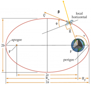
where [latex]\theta[/latex] is the angle between the [latex]\vec{R}[/latex] and [latex]\vec{V}[/latex] vectors, which can be related to the flight path angle by [latex]\phi = 90 - \theta[/latex]. Hence in equation (29):
(29)
[latex]\large \vec{R} \cdot \vec{V} = RV\sin\phi[/latex]
If the satellite is travelling from perigee to apogee, the angle between the [latex]\vec{R}[/latex] and [latex]\vec{V}[/latex] vectors is between 0° and 90° and [latex]\phi[/latex] is positive, hence sin [latex]\phi[/latex] is also positive. If the satellite is travelling from apogee to perigee, the angle between the [latex]\vec{R}[/latex] and [latex]\vec{V}[/latex] vectors is between 90° and 180° and [latex]\phi[/latex] is negative, hence sin [latex]\phi[/latex] is also negative. Thus the sign of the dot product, [latex]\vec{R} \cdot \vec{V}[/latex] provides a convenient way of determining which half plane the satellite is in.
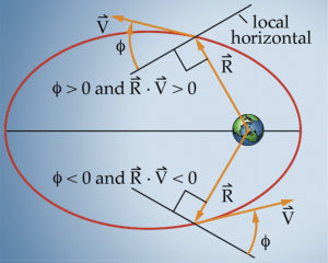
The half plane check for true anomaly thus becomes in equation (30):
(30)
If [latex]\large \vec{R} \cdot \vec{V}[/latex] < 0 then 180 < [latex]\large \nu[/latex] < 360 degrees.
If the satellite is at perigee, then the true anomaly is 0 and if the satellite is at apogee, then the true anomaly is 180°.
Note [latex]\nu[/latex] is not defined if the orbit is circular, or has an eccentricity of 0, since there is no perigee in a circular orbit.
The Classical Orbital Elements are summarized in the table below:
| Element | Name | Description | Range of values | Undefined | ||
| a | Semi-major Axis | Orbital Size
[latex]a = \frac{\mu}{2\epsilon}[/latex] |
Depends on Orbit Type | Never | ||
| e | Eccentricity | Orbit Shape
[latex]\small\vec{e} =\frac{1}{\mu}[(V^{2} - \frac{\mu}{R})\vec{R} - (\vec{R} \cdot \vec{V})\vec{V}][/latex] [latex]\vec{e} =\frac{1}{\mu}(\vec{V} \times \vec{h})- \frac{\vec{R}}{\left| \vec{R} \right|}[/latex] |
Depends on Orbit Type | Never | ||
| i | Inclination | Orbital Tilt
[latex]i = \cos^{-1}(\frac{h_{k}}{h})[/latex] |
[latex]0 \le i \le 180[/latex] | Never | ||
| [latex]\Omega[/latex] | Right Ascension of Ascending Node (RAAN) |
Orbital Swivel [latex]\Omega = \cos^{-1}(\frac{n_{i}}{n})[/latex] If [latex]n_{j} \lt 0[/latex] then [latex]180 \lt \Omega \lt 360[/latex]
|
[latex]0 \le \Omega \lt 360[/latex] | When i = 0 or 180 degrees (equatorial orbit) | ||
|
[latex]\Omega[/latex] |
Argument of Perigee |
Orbit Orientation [latex]\omega = cos^{-1}(\frac{\vec{n} \cdot\vec{e}}{ne})[/latex] If [latex]e_{k} \lt 0[/latex] then [latex]180 \lt \omega \lt 360[/latex] |
[latex]0 \le \omega \lt 360[/latex] | When i = 0 or 180 degrees (equatorial orbit) or e = 0 (circular orbit) | ||
| [latex]\nu[/latex] | True Anomaly |
Location of the Satellite [latex]\nu = \cos^{-1}(\frac{\vec{e} \cdot \vec{R}}{eR})[/latex] If [latex]\vec{R} \cdot \vec{V} \lt 0[/latex] then [latex]180 \lt \nu \lt 360[/latex] |
[latex]0 \le \nu \lt 360[/latex] | When e = 0 (circular orbit) |
In the next section, we will address what to use when one or more of the Classical Orbital Elements are not defied. But first, work through this example problem to see how well you understand the concepts from this section. The answers and solutions are at the end of this chapter.
EXAMPLE 1
[latex]\large \vec{R} = 0\hat{I} + 0\hat{J} + 10,000\hat{K}[/latex]km
[latex]\large \vec{V} = 6\hat{I} + 0\hat{J} + 0\hat{K}[/latex] km/s
Answer the following questions:
- Where is the satellite currently?
- What is the flight path angle at the satellite’s current position?
- What is the orbit’s specific angular momentum?
- What is the orbit’s semi-major axis?
- What is the orbit’s eccentricity?
- What is its inclination, i?
- What is its RAAN, [latex]\Omega[/latex]?
- What is its argument of perigee, [latex]\omega[/latex]?
- What is the satellite’s true anomaly, [latex]\nu[/latex]?
ALTERNATE ORBITAL ELEMENTS
As indicated in the table above, there are situations where one or more of the COEs are not defined. What do we do in those situations? In those cases, we use one of the alternate orbital elements.
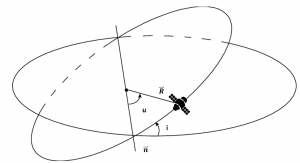
Argument of latitude, u
When a satellite is in a circular orbit, its argument of perigee, [latex]\omega[/latex], and true anomaly, [latex]\nu[/latex], are not defined. In this case, we use the argument of latitude, u, which indicates the location of the satellite in the orbit. It is the angle measured between the ascending node vector, [latex]\vec{n}[/latex], and the position vector to the satellite, [latex]\vec{R}[/latex] , as shown in the figure below.
Hence, argument of latitude is given by:
[latex]\large \cos u = \frac{\vec{n} \cdot\vec{R}}{nR}[/latex]
Or
[latex]\large u = \cos^{-1} (\frac{\vec{n} \cdot \vec{R}}{nR})[/latex]
Argument of latitude can take any value between 0° and 360° so a half plane check is needed. As can be seen in the figure above, if the kth component of the position vector is negative, then argument of perigee is in the second half plane. This can be written mathematically as:
If Rk < 0 then 180 < u < 360 degrees.
In the figure above, argument of latitude is about 25°.
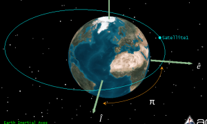
Longitude of Perigee
When a satellite is in an equatorial orbit, it has no ascending node vector, [latex]\vec{n}[/latex], and hence RAAN, [latex]\Omega[/latex] and argument of perigee, [latex]\omega[/latex] are undefined. In this case, we use the longitude of perigee, [latex]\Pi[/latex] which indicates the orientation of the orbit, or where its perigee is located. It is the angle measured between the vernal equinox direction, [latex]\hat{I}[/latex] and the eccentricity vector, [latex]\vec{e}[/latex], which points to perigee. The longitude of perigee is show in the figure below.
Hence, longitude of perigee is given by:
[latex]\large\cos\Pi = \frac{\hat{I} \cdot \vec{e}}{e}[/latex]
Or
[latex]\large \Pi = \cos^{-1}(\frac{e_{i}}{e})[/latex]
Longitude of perigee can take any value between 0° and 360° so a half plane check is needed. As can be seen in the figure above, if the jth component of the eccentricity vector is negative, then longitue of perigee is in the second half plane. This can be written mathematically as:
If ej < 0 then 180 < [latex]\large \Pi[/latex] < 360 degrees.
In the figure above, longitude of perigee is about 90°.
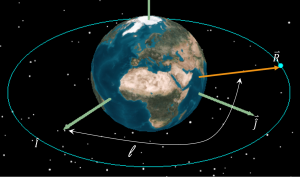
True Longitude
When a satellite is in an equatorial orbit and is circular, it has no ascending node vector, [latex]\vec{n}[/latex], and hence RAAN, [latex]\Omega[/latex], argument of perigee, [latex]\omega[/latex], and true anomaly, [latex]\nu[/latex], are undefined. In this case, we use the true longitude, l, which indicates the location of the satellite in its orbit. Thus, It is the angle measured between the vernal equinox direction, [latex]\hat{I}[/latex] and the position vector, [latex]\vec{R}[/latex]. The true longitude is shown in the figure below:
Hence, true longitude is given by:
[latex]\large \cos l = \frac{\hat{I} \cdot \vec{R}}{R}[/latex]
Or
[latex]\large l =\cos^{-1} (\frac{R_{i}}{R})[/latex]
True longitude can take any value between 0° and 360° so a half plane check is needed. As can be seen in the figure above, if the jth component of the position vector is negative, then true longitude is in the second half plane. This can be written mathematically as:
If Rj < 0 then 180 < [latex]\large l[/latex] < 360 degrees.
In the figure above, true longitude is about 115°.
The Alternate Orbital Elements are summarized in the table below.
| Element | Name | Description | Range of Values | When To Use |
| u | Argument of Latitude |
[latex]u = \cos^{-1}(\frac{\vec{n} \cdot \vec{R}}{nR})[/latex] If Rk<0 then 180 < u < 360 deg |
[latex]0 \le u \lt 360[/latex] | [latex]e = 0[/latex] and [latex]i \not= 0[/latex] |
| [latex]\Pi[/latex] | Longitude of Perigee |
[latex]\Pi = \cos^{-1}(\frac{e_{i}}{e})[/latex]
If ej < 0 then 180 < [latex]\Pi[/latex] < 360 deg |
[latex]0 \le \Pi \lt 360[/latex]
|
[latex]i = 0[/latex] and [latex]e \not= 0[/latex] |
| [latex]l[/latex] | True longitude |
[latex]l = \cos^{-1}(\frac{R_{i}}{R})[/latex] If Rj < 0 then 180 < [latex]l[/latex] < 360 deg |
[latex]0 \le l \lt 360[/latex]
|
[latex]i = 0[/latex] and [latex]e = 0[/latex] |
To see if you understand the alternate COEs, complete examples 2 and 3. The answers and solutions are at the end of this chapter.
EXAMPLE 2
[latex]\large \vec{R} = 10,000 \hat{I} + 0 \hat{J} + 0\hat{K}[/latex] km
[latex]\large \vec{V} = 0 \hat{I} + 4.464 \hat{J} - 4.464\hat{K}[/latex] km/s
Answer the following questions:
- Where is the satellite currently?
- What is the flight path angle at the satellite’s current position?
- What is the orbit’s specific angular momentum?
- What are the orbit’s orbital elements?
EXAMPLE 3
[latex]\large \vec{R} = 0 \hat{I} - 7,000 \hat{J} + 0\hat{K}[/latex] km
[latex]\large \vec{V} = 9\hat{I} + 0 \hat{J} + 0\hat{K}[/latex] km/s
Answer the following questions:
- Where is the satellite currently?
- What is the flight path angle at the satellite’s current position?
- What is the orbit’s specific angular momentum?
- What are the orbit’s orbital elements?
Complete this quick quiz in order to see how well you understand the concepts from this section.
In the next section, we will continue considering the “big picture” of how to determine where a satellite is located in orbit given earth-based observations. This will introduce us to two more coordinate systems, PQW and SEZ.
OPTIONAL MATERIAL
ORBITAL VISUALIZATION TOOLS
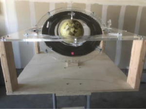
As part of a first astrodynamics class, the author often uses 3-D orbit visualization tools. A custom-designed and built orbital demonstrate at use at the University of Colorado, Colorado Springs is shown below.
However, since it is not possible for every student to have a large orbital demonstrator, we provide a hand-held orbital element model, or “whiz wheel”, to help students with the visualization of orbits. A 3-D printed “whiz wheel” is shown below:
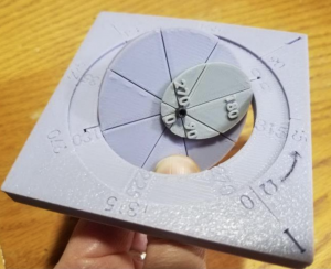
This device has the capability of demonstrating the following:
1. The physical characteristics of the COEs including how they are measured relative to the principle axes and fundamental plane of the geocentric-equatorial coordinate system, and in which direction the COEs are measured.
2. The effect that change in the values of the COEs will have on the orbit.
3. The resulting ground tracks caused by the earth rotating on its axis under the orbit fixed in space.
Take this quick quiz to see if you have a good understanding of orbital visualization.
When the author taught at the US Air Force Academy in the Department of Astronautics, cardboard paper versions of whiz wheels were used as an orbital visualization tool. When 3-D printing technology came along, it was a perfect candidate for development of a more durable tool, while keeping it small enough to still be handheld and easily carried in a backpack.
For instructions on how to build your own whiz wheel out of cardboard paper and some examples on how to use it, see the following attachments:
10 New whiz_wheel (ivory print at 74-76 percent)
3D files:
https://drive.google.com/file/d/1d3IDyytBZpwbwhFpYIB5rT6c0JAiNfR4/view?usp=drive_link
PROGRAMMING THE ORBITAL ELEMENTS
- Given position and velocity vectors for any earth satellite, write a program to calculate the COEs. Your output should be formatted to clearly indicate the orbit type (circular, elliptical, parabolic, hyperbolic, and/or equatorial) as well as the COEs or alternate COEs.
For practical purposes, consider orbits:
- circular if eccentricity < .001
- parabolic if < .001
- equatorial if inclination < .001°
- Run your program for the following cases. Include an accompanying set of hand calculations for cases 2 and 5. All units are in kms and seconds.
Case 1
[latex]\vec{R} = -424.0961\hat{I} - 369.963 \hat{J} + 7757.78\hat{K}[/latex]
[latex]\vec{V} = -1.364721 \hat{I} + 7.9109 \hat{J} + 2.86777\hat{K}[/latex]
Case 2
[latex]\large \vec{R} = 10000\hat{I} + 0 \hat{J} + 0\hat{K}[/latex]
[latex]\large \vec{V} = 0 \hat{I} + 4.464 \hat{J} - 4.464\hat{K}[/latex]
Case 3
[latex]\large \vec{R} = -12208 \hat{I} - 25698 \hat{J} - 8680\hat{K}[/latex]
[latex]\large \vec{V} = 4\hat{I} + 0 \hat{J} - 6\hat{K}[/latex]
Case 4
[latex]\large \vec{R} = 19455 \hat{I} + 8305 \hat{J} + 0\hat{K}[/latex]
[latex]\large \vec{V} = 3\hat{I} + 3 \hat{J} + 0\hat{K}[/latex]
Case 5
[latex]\large \vec{R} = 24912.16\hat{I} + 0 \hat{J} + 0\hat{K}[/latex]
[latex]\large \vec{V} = 0 \hat{I} + 4 \hat{J} + 0\hat{K}[/latex]
Case 6
[latex]\large \vec{R} = 7199\hat{I} + 9700\hat{J} + 15940\hat{K}[/latex]
[latex]\large \vec{V} = 4.464 \hat{I} + 4.464 \hat{J} + 0\hat{K}[/latex]
Solutions to Cases 1 and 5 are provided.
SOLUTIONS TO EXAMPLES:
***EXAMPLE 1 SOLUTION***
[latex]\large \vec{R} = 0 \hat{I} + 0 \hat{J} + 10,000\hat{K}[/latex] km
[latex]\large \vec{V} = 6 \hat{I} + 0 \hat{J} + 0\hat{K}[/latex] km/s
Answer the following questions:
- Where is the satellite currently? Over the north pole. You know this because the position vector has only a positive [latex]\hat{K}[/latex] component.
2. Flight path angle, [latex]\large \phi[/latex] = 0. We know this because the position and velocity vectors are perpendicular (their dot product is zero).
3. Specific angular momentum vector, [latex]\large \vec{h}[/latex]
[latex]\large \vec{h} = \vec{R} \times \vec{V}[/latex]= [latex]\begin{vmatrix} \hat{I} & \hat{J} & \hat{K}\\ 0 & 0 & 10,000 \\ 6 & 0 & 0 \end{vmatrix}[/latex] = [latex]60,000 \hat{J}[/latex]km2/s
[latex]\large \vec{h}[/latex]= 60,000 [latex]\hat{J}[/latex] km2/s
4. Semi-major axis, a
[latex]\large \varepsilon = \frac{V^{2}}{2} - \frac{\mu}{R} = \frac{6^{2}}{2} - \frac{389600.5}{10000} = -21.86[/latex] km2/s2
[latex]\large a = -\frac{\mu}{2\varepsilon} = -\frac{398600.5}{2(-21.68)} = 9117[/latex] km
a = 9117 km
5. Eccentricity, e
In this example, we will look at three methods to find e:
a. Method 1. Use the long form of the eccentricity vector equation; however, in this case it simplified a lot since [latex]\large \vec{R} \cdot\vec{V}[/latex].
[latex]\large \vec{e} = \frac{1}{\mu}[(V^{2} - \frac{\mu}{R}) \vec{R} - (\vec{R} \cdot \vec{V})\vec{V}] = \frac{1}{389600.5}[(6^{2} - \frac{398600.5}{10000})10000\hat{K} -0] = -0.0968\hat{K}[/latex]
[latex]\large e = \vec{e} = 0.0968[/latex]
e = 0.0968
b. Method 2. Use the dot product form of the eccentricity vector equation.
[latex]\large \vec{e} = \frac{1}{\mu}(\vec{V} \cdot \vec{h}) - \frac{\vec{R}}{\left| \vec{R} \right|}[/latex]
[latex]\large \vec{V} \times \hat{h} = \begin{vmatrix} \hat{I} & \hat{J} & \hat{K}\\ 6 & 0 & 0 \\ 0 & 60000 & 0 \end{vmatrix} = 360,000\hat{K}[/latex]
[latex]\large \hat{e} = \frac{1}{398600.5}(360,000\hat{K})- \frac{10000\hat{K}}{10000} = -0.0968\hat{K}[/latex]
e = 0.0968
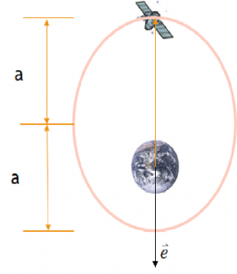
c. Method 3. Use radius of apogee to determine the magnitude of e. This takes a little thought, but once you have done these a few times it becomes more and more obvious. Follow this logic:
i. Since [latex]\large \vec{R} \cdot \vec{V}[/latex], the two vectors are perpendicular. Hence, the flight path angle will be zero, which only occurs at two points in an elliptical orbit: apogee and perigee.
ii. Since the semi-major axis, a = 9117 km and the position vector is currently at a magnitude of 10,000 km, the satellite must be at apogee as can be seen in the figure below:
Since Ra = a(1 + e)
10000 = 9117 (1 + e)
e = 10000/9117 – 1
e = 0.0968
6. What is its inclination, i?
Since the position vector has only a [latex]\hat{K}[/latex] component,
i = 90 degrees
Alternately, you may calculate this using the equation:
[latex]\large i = \cos^{-1}(\frac{h_{k}}{h})[/latex]
From 3,
[latex]\large \vec{h} = 60,000 \hat{J}[/latex] km2/s
The k component of [latex]\large \vec{h}[/latex] is 0, hence,
i = cos-1(0) = 90 degrees
i = 90 degrees
7. What is its RAAN, [latex]\Omega[/latex]?
Since the velocity vector has only an [latex]\large \hat{I}[/latex] component, by inspection (see Figure “Example 1 Orbit” under #1),
[latex]\large \Omega[/latex] = 180 degrees
Alternately, you may calculate RAAN using the equation:
[latex]\large \Omega = \cos^{-1}(\frac{n^{i}}{n})[/latex]
First, you will need to find the ascending node vector = [latex]\large \vec{n} = \hat{K} \times \vec{h}[/latex]
[latex]\large \hat{K} \times \vec{h} = \begin{vmatrix} \hat{I} & \hat{J} & \hat{K}\\ 0 & 0 & 1 \\ 0 & 60000 & 0 \end{vmatrix} = - 60,000\hat{I}[/latex]
[latex]\large \omega[/latex] = cos-1(-60000/60000) = cos-1(-1)
[latex]\large \omega[/latex] = 180 degrees
8. What is its argument of perigee, [latex]\large \omega[/latex]?
Since the ascending node vector, [latex]\large \vec{n}[/latex], only has a negative[latex]\hat{I}[/latex] component and the eccentricity vector points through the south pole,
[latex]\large \omega[/latex] = 270 degrees
Alternately, you may calculate argument of perigee using the equation:
[latex]\large \omega = \cos^{-1}(\frac{\vec {n} \cdot \vec{e}}{ne})[/latex]
since [latex]\large \vec{n} = -60000 \hat{I}[/latex]
and [latex]\large \vec{e} = -0.0968 \hat{K}[/latex]
Their dot product is equal to zero. Hence
[latex]\large \omega[/latex] = cos-1(0) = 90 degrees or 270 degrees
However, since, ek<0,
[latex]\large \omega[/latex] = 270 degrees
9. What is the satellite’s true anomaly, [latex]\large \nu[/latex]?
Since the satellite is currently at apogee,
[latex]\large \nu[/latex] = 180 degrees
Alternately, you may calculate true anomaly using the equation:
[latex]\large \nu = \cos^{-1}(\frac{(-0.0968)(10000)}{(0.0968)(10000)})[/latex]
[latex]\large \nu[/latex] = cos-1(-1)
[latex]\large \nu[/latex] = 180 degrees
***EXAMPLE 2 SOLUTION***
[latex]\large \vec{R}= 10,000 \hat{I} + 0\hat{J} + 0\hat{K}[/latex] km
[latex]\large \vec{V} = 0\hat{I} + 4.464\hat{J} - 4.464\hat{K}[/latex] km/s [latex]\vec{V} = 0\hat{I} + 4.464\hat{J} - 4.464\hat{K}[/latex] km/s
1. Where is the satellite currently? Over the equator at the descending node.
2. What is the flight path angle at the satellite’s current position? 0 (position and velocity vectors are perpendicular)
3. What is the orbit’s specific angular momentum?
[latex]\large \vec{h} = \vec{R} \times \vec{V} = \begin{vmatrix} \hat{I} & \hat{J} & \hat{K}\\ 10000 & 0 & 0 \\ 0 & 4.464 & 4.464 \end{vmatrix} = - 44,640\hat{J} + 44,640\hat{K}[/latex] km2/s
[latex]\large \vec{h} = 0\hat{I} + 44,640 \hat{J} + 44,640 \hat{K}[/latex] km2/s
4. What are the orbit’s orbital elements?
Semi-major axis, a
[latex]\large V = \left| \vec{V} \right| = \sqrt{4.464^{2} + 4.464^{2}} \frac{km}{s}[/latex]
V = 6.313 km/s
[latex]\large R = \left| \vec{R} \right| = 10,000[/latex] km
so [latex]\large \varepsilon = \frac{V^{2}}{2} - \frac{\mu}{R} = \frac{6.313^{2}}{2} - \frac{398600.5}{10000} = -19.93 \frac{km}{s}[/latex]
and [latex]\large a = -\frac{\mu}{2\varepsilon} = -\frac{398600.5}{2 \times(-19.93)}[/latex]
a = 10000 km
Thus, this is a circular orbit.
eccentricity, e
Since this is a circular orbit, e = 0
inclination, i
By inspection using a drawing or visualization tool (introduced later), it can be deduced that:
i = 45 degrees
Alternately, it can be calculated by [latex]\large \cos i = \frac{\vec{h} \cdot \hat{K}}{hK}[/latex]
From part 3, [latex]\large h = \left| \vec{h} \right| = \sqrt{44640^{2} + 44640^{2}} \frac{km^{2}}{s}[/latex]
h = 63130 km2/s
So [latex]\large \cos i = \frac{44640}{63130} = \frac{1}{\sqrt{2}}[/latex]
i = 45 degrees
Right Ascension of Ascending Node (RAAN), [latex]\large \Omega[/latex]
Again, by inspection it can be determined that:
[latex]\large \Omega[/latex] = 180 degrees
Alternatively, it can be calculated by [latex]\large \cos \Omega = \frac{\hat{I} \cdot \hat{n}}{In}[/latex]
Where [latex]\large \vec{n} = \hat{K} \times \vec{h}[/latex]
[latex]\large \vec{n} = \begin{vmatrix} \hat{I} & \hat{J} & \hat{K}\\ 0 & 0 & 1 \\ 0 & 44640 & 44640 \end{vmatrix}[/latex]
[latex]\large \vec{n} = -44640\hat{I} + 0\hat{J} + 0\hat{K}[/latex] km2/s
so [latex]\large \cos \Omega = \frac{-44640}{44640} = -1[/latex]
[latex]\large \Omega[/latex] = 180 degrees
Now since this is a circular orbit, there is no argument of perigee, so we must use an alternate COE.
Argument of latitude, u
u is measured from the ascending node vector, [latex]\large \vec{n}[/latex] to the position vector, [latex]\large \vec{R}[/latex]
Again, by a good drawing or visualization tool, it can be seen by inspection that:
u = 180 degrees
Alternatively, it can be calculated by [latex]\large \cos u = \frac{\vec{n} \cdot\vec{R}}{nR}[/latex]
From before, we found:
[latex]\large \vec{n} = -44640\hat{I} + 0\hat{J} + 0\hat{K}[/latex] km2/s
and since [latex]\large \vec{R} = 10,000\hat{I} + 0\hat{J} + 0\hat{K}[/latex] km
so [latex]\large \cos u = \frac{(-44640)(10000)}{(44640)(10000)}[/latex]
u = 180 degrees
***EXAMPLE 3 SOLUTION***
[latex]\large \vec{R} = 0\hat{I} - 7000\hat{J} + 0\hat{K}[/latex] km
[latex]\large \vec{V} = 9\hat{I} + 0\hat{J} + 0\hat{K}[/latex] km/s
Answer the following questions:
- Where is the satellite currently?
About all you can tell at this point is that the satellite is over the equator at either apogee, perigee, or in a circular orbit. There are no [latex]\hat{K}[/latex] components in either the velocity or position vectors, so this must be an equatorial orbit.
2. What is the flight path angle at the satellite’s current position? Zero
We observe that the [latex]\vec{R}[/latex] and [latex]\vec{V}[/latex] are perpendicular, so at that instant the flight path angle is zero, hence at apogee, perigee (in an elliptical orbit) or in a circular orbit.
3. What is the orbit’s specific angular momentum?
[latex]\large \vec{h} = \vec{R} \times \vec{V}[/latex]
[latex]\large \vec{h} = \begin{vmatrix} \hat{I} & \hat{J} & \hat{K}\\ 0 & -7000 & 0 \\ 9 & 0 & 0 \end{vmatrix}[/latex]
[latex]\large \vec{h} = 63000\hat{K}[/latex] km2/s
4. What are the orbit’s orbital elements?
Semi-major axis, a
[latex]\large \varepsilon = \frac{V^{2}}{2} - \frac{\mu}{R} = -\frac{\mu}{2a}[/latex]
so
[latex]\large \varepsilon = \frac{9^{2}}{2} - \frac{398600.5}{7000} = -16.44[/latex] km2/s2
[latex]\large a = -\frac{\mu}{2\varepsilon}[/latex] so [latex]a = -\frac{398600.5}{7000}[/latex]
a = 12120 km
Eccentricity, e
In this example, we will look at three methods to find e.
a. Method 1. Use the long form of the eccentricity vector equation; however, in this case it simplified a lot since [latex]\vec{R} \cdot \vec{V} = 0[/latex].
[latex]\large \vec{e} = \frac{1}{\mu}[(V^{2}-\frac{\mu}{R})\vec{R} - (\vec{R} \cdot\vec{V})\vec{V}] = -.422\hat{J}[/latex]
[latex]\large e = \left| \vec{e} \right| = 0.422[/latex]
e = 0.422
b. Method 2. Use the cross product form of the eccentricity vector equation.
[latex]\large \vec{e} = \frac{1}{\mu}(\vec{V} \times \vec{h}) - \frac{\vec{R}}{\left| \vec{R} \right|}[/latex]
where
[latex]\large \vec{V} \times \vec{h} = \begin{vmatrix} \hat{I} & \hat{J} & \hat{K}\\ 9 & 0 & 0 \\ 0 & 0 & 63000 \end{vmatrix} = -567000\hat{J}[/latex]
so
[latex]\large \vec{e} = \frac{1}{398600.5}(-567000\hat{J}) - \frac{(-7000\hat{J})}{7000}[/latex]
[latex]\large \vec{e} = -1.4225\hat{J} + 1\hat{J}[/latex]
[latex]\large \vec{e} = -0.4225\hat{J}[/latex]
e = 0.422, which is the same result we had previously.
c. Method 3. Use radius of apogee to determine the magnitude of e. This takes a little thought, but once you have done these a few times it becomes more and more obvious. Follow this logic:
i. Since [latex]\large \vec{R} \times \vec{V} = 0[/latex], the two vectors are perpendicular. Hence, the flight path angle will be zero, which only occurs at two points in an elliptical orbit: apogee and perigee.
ii. Since the semi-major axis, a = 12120 km and the position vector is currently at a magnitude of 7000 km, the satellite must be at perigee as can be seen in the figure below.
Since Ra = a(1 – e)
7000 = 12120 (1 – e)
e = 1 – 7000/12120
e = 0.422
inclination, i
By inspection using a drawing or visualization tool and since there are no [latex]\widehat{K}[/latex] components in either the velocity or position vectors, so this must be an equatorial orbit, it can be deduced that:
i = 0 degrees
Alternately, you could calculate it by using:
[latex]\large \cos i = \frac{\vec{h} \cdot \hat{K}}{hK}\large[/latex]
Since from part 3) [latex]\large \vec{h}[/latex] = 63000 [latex]\hat{K}[/latex] km2/s
[latex]\large \cos i = \frac{63000}{63000} = 1 \large[/latex]
so i = 0 degrees
Longitude of Perigee, [latex]\large \Pi[/latex]
Since there is no ascending node, there is no right ascension of ascending node [latex]\Omega[/latex]. However, this is an eccentric orbit so it has a perigee and since longitude of perigee is measured from the [latex]\hat{I}[/latex]vector to perigee, by inspection, we can deduce:
[latex]\large \Pi[/latex] = 270 degrees
Alternatively you could calculate it using:
[latex]\large \cos \Pi = \frac{\hat{I} \cdot \hat{e}}{e}[/latex]
From above, [latex]\large \vec{e}[/latex] = -0.4225 [latex]\hat{J}[/latex]
cos[latex]\large \Pi[/latex] = 0
so [latex]\large \Pi[/latex] = 90 degrees or 270 degrees
However, our quadrant check, if ej < 0 then 180 < [latex]\large \Pi[/latex] < 360 deg, tells us [latex]\large \Pi[/latex] must be in the second half plane, hence,
[latex]\large \Pi[/latex] = 270 degrees
True Anomaly, [latex]\large \nu[/latex]
Since the satellite is currently at perigee,
[latex]\large \nu[/latex] = 0 degrees
Alternately, you may calculate true anomaly using the equation:
[latex]\large \cos \nu = \frac{\vec{e} \cdot \vec{R}}{eR}[/latex]
[latex]\large \cos i = \frac{63000}{63000} = 1[/latex]
[latex]\large \nu[/latex] = cos-1(1)
[latex]\large \nu[/latex] = 0 degrees
REFERENCES
Bate, R. R., Mueller, D. D., White, J. E., & Saylor, W. W. (1971). Fundamentals of astrodynamics. Mineola (N.Y.): Dover Publications.
Exo Cruiser (2016, March). Where is the Solar System Zero? dodlithr.blogspot.com
Martin, Reeve. (2009, June 28). First point of Aries. https://stargazerslounge.com/topic/44684-first-point-of-aries/
Rune, Signa. (2014, July 18). The two-body equation of motion. https://www.slideserve.com/signa/the-two-body-equation-of-motion
Sanad, Ibrihim. (2013, January). (Pdf) Design of Remote Sensing Satellite Orbit. (n.d.). https://www.researchgate.net/publication/311486304_Design_of_Remote_Sensing_Satellite_Orbit
Strimel, Greg & Bartholomew, Scott & Kim, Eunhye. (2017). Engaging Children in Engineering Design Through the World of Quadcopters. Children’s Technology and Engineering Journal. 21. 7-11.
Sellers, Jerry Jon. (2005). Understanding Space: An Introduction to Astronautics, 3rd edition. McGraw-Hill.
Siegenthaler, Kenneth, David Barnart, Jerry Sellers, James White and Tim White (2004). Educational Methods/Aids Used in the
Astronautics Core Course at the United States Air Force Academy. Proceedings of the 2004 American Society for Engineering
Education Annual Conference & Exposition, American Society for Engineering Education.”
Taghinivarami, Khodayar (2016, July). (Pdf) Rotational Evolution of Low-Mass Stars in Close Binaries. https://www.researchgate.net/publication/309727000_Rotational_Evolution_of_Low-Mass_stars_in_close_binaries
United States Air Force Academy Department of Astronautical Engineering. (n.d.) Astro 310 Whiz Wheel.
United States Air Force Academy Department of Astronautical Engineering (n.d.) Whiz Wheel Examples.
Media Attributions
- Figure 1: Two-Body-EOM-Geometry © John Siegenthaler is licensed under a Public Domain license
- Figure 2: Example 3D Coordinate Frame (Edited) © Nav Ganti is licensed under a CC0 (Creative Commons Zero) license
- Figure 3: Geocentric-Equatorial Coordinate System (Edited) © FAA is licensed under a Public Domain license
- Figure 4: Aries – My (Waid) Birth Sign © Jess Waid is licensed under a CC BY-SA (Attribution ShareAlike) license
- Figure 5: First Point of Aries © Kwantus is licensed under a CC BY-SA (Attribution ShareAlike) license
- Figure 6: Six Degrees of Freedom © Strimel, Greg & Bartholomew, Scott & Kim, Eunhye is licensed under a CC0 (Creative Commons Zero) license
- Figure 7: Parameters Associated With an Elliptical Orbit © Lynnane George is licensed under a Public Domain license
- Figure 8: Two-Body EOM Geometry (Edited) © John Siegenthaler is licensed under a Public Domain license
- Figure 9: The Geocentric Equatorial Coordinate Frame © FAA is licensed under a Public Domain license
- Figure 10: Angle Between Two Vectors © Lynnane George is licensed under a Public Domain license
- Figure 11: Types of Orbits and Their Inclination Table © FAA is licensed under a Public Domain license
- Figure 12: Right Ascension of the Ascending Node, Omega © FAA is licensed under a Public Domain license
- Figure 13: Twist: Right Ascension of the Ascending Node, Omega © London is licensed under a CC0 (Creative Commons Zero) license
- Figure 14: Various Terms in Relation to Orbits of Celestial Bodies (Edited) © Lasunncty is licensed under a CC BY-SA (Attribution ShareAlike) license
- Figure 15: Argument of Perigee, Omega © FAA is licensed under a Public Domain license
- Figure 16: Argument of Perigee (270) © Air University is licensed under a CC0 (Creative Commons Zero) license
- Figure 17: Parameters Associated With an Elliptical Orbit © Lynnane George is licensed under a Public Domain license
- Figure 18: Half Plane Check for True Anomaly. © Lynnane George is licensed under a Public Domain license
- Figure 19: Argument of Latitude © Lynnane George is licensed under a Public Domain license
- Figure 20: Longitude of Perigee Model © Lynnane George is licensed under a Public Domain license
- Figure 21: True Longitude of Perigee Model © Lynnane George is licensed under a Public Domain license
- Figure 22: Classroom Orbital Demonstrator Snapshot © Lynnane George is licensed under a Public Domain license
- Figure 23: A 3-D “Whiz Wheel” Orbital Demonstrator © Lynnane George is licensed under a Public Domain license
- Figure 24: Satellite Over the North Pole Model © Lynnane George is licensed under a Public Domain license
- Figure 25: Satellite at Apogee Point Model © Lynnane George is licensed under a Public Domain license
- Figure 26: Satellite at Perigee Point Model © Lynnane George is licensed under a Public Domain license
