2 Chapter 2 – Orbit Geometry
ORBITS AS CONIC SECTIONS
In Chapter 1, the Two Body Equation of Motion was developed and we discussed how the elliptical orbit was one possible solution. In general, however, the solution can be any of the four conic sections: circles, ellipses, parabolas and hyperbolas. We will start this chapter with a discussion of how a satellite gets into orbit and relate it to the conic sections. We will then review the elliptical orbit and its parameters and then extend these results to consider the other conic sections.
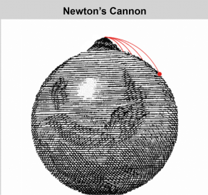
First, how does a satellite get into orbit? Imagine you are at the top of a mountain and start firing a cannon from it. We can think of the cannonball as a projectile, an object that, when it is set in motion, continues in its path by its own inertia and is influenced only by the downward force of gravity. The horizontal motion of the projectile is the result of the tendency of any object in motion to remain in motion at a constant velocity. The vertical motion of the projective, or cannonball, is influenced by the gravitational acceleration, g, pulling downward. The horizontal and vertical motions are independent, hence, the faster you fire the cannonball, the farther it will go. As an example, try the Newton’s Cannon simulator below (Figure 1). In this simulation, the cannon was fired at 3000 m/s, 4000 m/s, 5000 m/s and 6000 m/s. Each time the cannonball goes a little farther before hitting the earth. Try the simulator yourself and see what happens! (Schroeder, 2020).
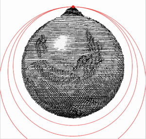
Since the earth is approximately spherically shaped (we will find out later that this it not entirely true), its surface drops about 5 meters for every 8 km the cannonball travels horizontally. So, if we fire the cannonball faster and faster (assuming no air resistance), its path would eventually match the rate of curvature of the earth. Here are the results of the simulator firing the cannon at 7300 m/s, 7600 m/s, and 8000 m/s (Figure 2). You will notice that at the lower velocity, the orbit is nearly circular; however, as the cannonball is fired faster and faster, the orbital shape becomes more elliptical. In fact, as more and more horizontal velocity is added, the orbit will eventually become parabolic, then hyperbolic, eventually breaking away from the earth’s sphere of influence entirely. We will consider each of these types of orbits in this chapter.
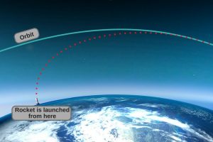
A rocket launches vertically to get as quickly as possible out of the earth’s thick atmosphere and minimize drag. However, you will notice that it begins to tilt horizontally and gradually increases this tilt until it achieves orbit around the earth. This technique of optimizing a trajectory of a rocket so that it attains the desired path is called a gravity turn, as demonstrated in Figure 3. This technique allows the rocket to use Earth’s gravity rather than its own fuel in order to change its direction. The fuel that the rocket saves can then be used to accelerate it horizontally in order to attain high speed and more easily enter into orbit.
ELLIPTICAL ORBITS
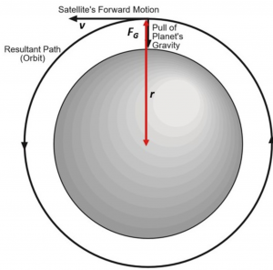
Kepler’s First Law said the orbits of the planets are ellipses. These are the most common orbits because one object is ‘captured’ and orbits another larger object, as seen in Figure 4. Not only do the planets and minor planets have elliptical orbits, most comets and binary stars also do. The velocity in elliptical orbits is always less than that needed to escape from the central object’s influence. Let us take a closer look at the geometry of an orbital ellipse, which we considered in Chapter 1, and describe each of its parameters more precisely.
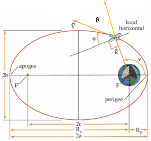
[latex]\vec{R}[/latex] = satellite position vector, measured from the center of the Earth
[latex]R[/latex] = the radius from the focus of the ellipse (center of the earth) to the satellite, or [latex]R=\left | \vec{R} \right |[/latex], the magnitude of the [latex]\vec{R}[/latex] vector
[latex]\vec{V}[/latex] = satellite velocity vector, tangent to the orbital path
[latex]V[/latex] = the magnitude of the [latex]\vec{V}[/latex] vector
[latex]F[/latex] and [latex]F'[/latex] = primary (occupied) and vacant (unoccupied) foci of ellipse
[latex]R_{p}[/latex]= Radius of periapsis (closest point) = Radius of perigee when the satellite is around the earth = a(1-e)
[latex]R_{a}[/latex]= Radius of apoapsis (farthest point) = Radius of apogee when the satellite is around the earth = a(1+e)
[latex]\large =\frac{R_{a}+R_{p}}{2}[/latex]
[latex]a[/latex] = semi-major axis
[latex]b[/latex] = semi-minor axis
[latex]2c[/latex] = the distance between the foci [latex]R_{a}-R_{p}[/latex]
[latex]e[/latex] = eccentricity, the ratio of the distance between the foci (2c) to the length of the ellipse (2a), or [latex]e=\frac{c}{a}[/latex]. Thus
[latex]\large e=\frac{R_{a}-R_{p}}{R_{a}+R_{p}}[/latex]
Eccentricity defines the shape of the conic section. For ellipses,
[latex]\large 0<e<1[/latex]
[latex]V[/latex] = true anomaly = the polar angle measured from perigee to the satellite position vector, [latex]\vec{R}[/latex], in the direction of satellite motion
[latex]\phi[/latex] = flight path angle, measured from the local horizontal to the velocity vector, [latex]\vec{V}[/latex].
When the satellite is traveling from perigee to apogee, the velocity vector will always be above the local horizon (gaining altitude) so [latex]\phi[/latex] > 0 for [latex]0° < V < 180°[/latex].
When travelling from apogee to perigee, the velocity vector will always be below the local horizon (losing altitude) so [latex]\phi[/latex] < 0 for [latex]180° < V < 360°[/latex].
At exactly apogee and perigee on an ellipse, the position and velocity vectors will be perpendicular so the velocity vector is parallel to the local horizon, hence [latex]\phi[/latex] = 0.
p = semi-latus rectum = the magnitude of the position vectors at [latex]V = 90[/latex] degrees and 270 degrees
Since ellipses are closed curves, an object in an ellipse repeats its path over and over. The time for a satellite to go once around its orbit is called the period. For a detailed derivation of the period equation (1), see Bate.
(1)
[latex]\large Period=2\pi \sqrt{\frac{a^3}{\mu}}[/latex] seconds
Let us review what we know about orbits so far before taking a look at special types of orbits.
-
- Conic sections are the only possible paths for an orbiting object governed by the ideal two body equation of motion.
- The focus of the conic section is the center of the central body.
- The specific mechanical energy, [latex]\varepsilon[/latex] is constant, so potential energy and kinetic energy are traded off according to the relationship (2).
(2)
[latex]\large \varepsilon = \frac{V^2}{2}-\frac{\mu}{R}=-\frac{\mu}{2}[/latex]
This relationship also tells us that the orbit size is fixed.
The velocity can then be found by rearranging this equation (2) to yield Equation 3:
(3)
[latex]\large V = \sqrt{2(\frac{\mu}{R} + \varepsilon)}[/latex]
4. The specific angular momentum (Equation 4),
(4)
[latex]\large \vec{h} = \vec{R} \times \vec{V}[/latex]
is constant, so the orbital plane is fixed in orientation. Also Equation 5 demonstrates
(5)
[latex]\large h = |\vec{h}| = RVsin\beta[/latex]
where [latex]\beta[/latex] is the angle between [latex]\vec{R}[/latex] and [latex]\vec{V}[/latex] so
(6)
[latex]\large h=RVcos\phi[/latex]
Recall at at apogee and perigee, [latex]\vec{R}[/latex] and [latex]\vec{V}[/latex] are perpendicular so since [latex]\phi[/latex] = 0 degrees,
(7)
[latex]\large h = R_{p}V_{p}[/latex]
and
(8)
[latex]\large h = R_{a}V_{a}[/latex]
Finally, from Chapter 1 we found another express for specific angular momentum (9),
(9)
[latex]\large h=\sqrt{\mu a(1-e^2)}[/latex]
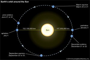
An example of an elliptical orbit is the earth’s orbit around the sun, as seen in Figure 5. It has a semi-major axis, a, of approximately 149,598,260 km and an eccentricity of 0.0174. This is a very low eccentricity, which results in only a 3% difference in the distance to the sun at perihelion and aphelion.
An example of a highly elliptical earth orbiting satellite is one travelling in a Molniya orbit (see Figure 6 below). It is a 12-hour orbit with semi-major axis, a, of 26,571 km, an eccentricity, e, of about 0.7. Its perigee is located in the Southern hemisphere and the satellite spends 11 hours, or about 92% of its time, in the northern hemisphere. We will study more about Molniya orbits when we discuss perturbations later in this book.
In the next section, we will consider a special case of elliptical orbits, known as circular orbits. But first, work through this example problem to see how well you understand the concepts from this section. The answers and solutions are at the end of this chapter.
EXAMPLE 1
The altitude of a satellite at perigee is 500 km and its orbital eccentricity is 0.1. Find:
a) The satellite’s altitude at apogee
b) The orbit’s specific mechanical energy, [latex]\varepsilon[/latex]
c) The magnitude of the orbit’s specific angular momentum, [latex]h[/latex]
d) The satellite’s speed at apogee
CIRCULAR ORBITS
The circular orbit is just a special case of an elliptical orbit (Figure 7), so the relationships for an elliptical orbit described above are valid.
The semi-major axis, a, is just it’s radius, or [latex]a = R[/latex] and the eccentricity of a circular orbit, [latex]e = 0[/latex]. This makes the period equation (10), in seconds,
(10)
[latex]\large P = 2\pi \sqrt{\frac{R^3}{\mu}}[/latex]
Also notice that the Velocity vector, [latex]\vec{V}[/latex], is always perpendicular to the Position vector, [latex]\vec{R}[/latex], so the flight path angle, [latex]\phi[/latex] is always equal to zero. We can calculate the speed required for a circular orbit of radius [latex]R[/latex] from the velocity equation (11):
(11)
[latex]\large V = \sqrt{2(\frac{\mu}{R} + \varepsilon)}[/latex]
Now we know
(12)
[latex]\large \varepsilon = -\frac{\mu}{2a} = -\frac{\mu}{2R}[/latex]
So now
(13)
[latex]\large V = \sqrt{2(\frac{\mu}{R} - \frac{\mu}{2R})} = \sqrt{2(\frac{\mu}{2R})}[/latex]
So the velocity of a satellite in a circular orbit simplifies to a constant:
(14)
[latex]\large V=\sqrt{\frac{\mu}{R}}[/latex]
Notice that the greater the radius of the circular orbit, the less speed is required to keep the satellite in this orbit. For a low altitude earth orbit, the circular speed is about 7.8 km/s, while the speed required to keep the moon in its orbit around the earth is only about 0.9 km/s.
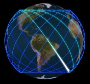
Although satellite orbits never have eccentricities exactly equal to zero, there are some satellites that come close. Global Positioning System, GPS, satellites provide navigation services worldwide. The satellite constellation’s main functions are to transmit radio-navigation signals and to store and retransmit navigation messages. These transmissions are controlled by highly stable atomic clocks that are on board the satellites. The constellation is designed so users will have at least four simultaneous satellites in view from any point on the earth’s surface at any time, as shown in Figure 8. The United Sates is committed to maintaining the availability of at least 24 operational GPS satellites 95% of the time. This means at any one time there are about 30 operational GPS satellites (ESA, 2020).
GPS satellites fly in medium space orbit (MEO) at an altitude of approximately 20,200 km, which results in a period of 12 hours and an orbital speed of 3.9 km/s. They are in 6 planes spaced equally (60 degrees apart) with four satellites in each. These orbits are nearly circular, with eccentricity less than 0.02.
Another example of a nearly circular orbit is the one used for the International Space Station, ISS (Figure 9). The ISS is a modular space station, or habitable artificial satellite, and is a multinational collaborative project involving five participating space agencies: NASA (United States), Roscosmos (Russia), JAXA (Japan), ESA (Europe), an CSA (Canada). It serves as a microgravity and space environment research laboratory and has been continuously occupied by humans since November 2000. The ISS flies in Low Earth Orbit (LEO) at an altitude of approximately 420 km, which results in a period of just over 90 minutes. This means the ISS circles the earth 15 to 16 times a day! Its orbit is also nearly circular, with an eccentricity of 0.0003 and an orbital speed of 7.7 km/s. It is at a relatively high orbital tilt of 51.6 degrees relative to earth’s equator, resulting in it passing over a large portion of the earth’s surface each day.
In the next section, we will consider parabolic orbits. But first, work through this example problem to see how well you understand the concepts from this section. The answers and solutions are at the end of this chapter.
EXAMPLE 2
A geostationary orbit, GEO, is one in which a satellite always remains above the same point on the earth’s equator. For a GEO satellite, the radial from the center of the earth to the satellite must have the same angular velocity as the earth itself, or a period of 24 hours.
1. Calculate the altitude of a GEO orbit.
2. Calculate the specific mechanical energy, [latex]\varepsilon[/latex], of a GEO satellite’s orbit.
3. Calculate the speed of a GEO satellite.
PARABOLIC ORBITS
Parabolic orbits (Figure 10) are rarely found in use, but they are important and interesting because they are the borderline case between the elliptical (closed) orbit and the hyperbolic (open) orbit.
The semi-major axis of a parabolic orbit is infinitely large, so an object traveling in a parabolic orbit is on a one-way trip to infinity and will never retrace the same path again. A unique property of a parabolic orbit is that the two arms of the parabola become more and more nearly parallel as they are extended further and further to the right of the focus.
Also, since the eccentricity of a parabolic orbit is 1, the radius to perigee equation used for elliptical orbits, [latex]R_{p} = a(1-e)[/latex], cannot be used so the more generic form will be used:
(15)
[latex]\large R_{p} = \frac{p}{1 + escov}[/latex]
Thus, for [latex]e = 1[/latex] and [latex]V = 0[/latex] degrees, this becomes:
(16)
[latex]\large R_{p} = \frac{p}{2}[/latex]
Of course, there is no apogee for a parabola and it may be thought of as an infinitely long ellipse.
Even though a planet’s gravitational field strength theoretically extends to infinity, its strength decreases rapidly with distance from the center body, such as the earth. Thus, there is a finite amount of kinetic energy that is needed to overcome the effects of gravity and allow an object to coast to an “infinite” distance without being pulled back toward the earth. The speed at which this occurs is called the escape speed, [latex]V_{esc}[/latex]. Theoretically, as the object’s distance from the earth approaches infinity, it’s speed approaches zero. This results in a total specific mechanical energy, [latex]\varepsilon = 0[/latex] for a parabolic orbit.
We can then calculate the speed necessary to escape by writing the energy equation (17) for this point:
(17)
[latex]\large \varepsilon = \frac{V^2_{esc}}{2} - \frac{\mu}{R} =0[/latex]
Thus
(18)
[latex]\large V_{esc}= \sqrt{\frac{2\mu}{R}}[/latex]
As you would expect, the farther away you are from the earth, the less speed it takes to escape from the remainder of the gravitational field. The escape speed from the surface of the earth is about 11.2 km/s, while from a point 6300 km above the surface, it will only take about 7.9 km/s.
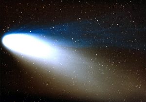
Although parabolic orbits are not used in practice, some comets approach parabolic orbits. For example, Comet McNaught, also known as the Great Comet of 2007 and given the designation C/2006 P1, is a non-periodic comet. It was discovered on 7 August 2006 by British-Australian astronomer Robert McNaught. It was the brightest comet in over 40 years and it was visible to the naked eye for observers in the Southern Hemisphere in January and February 2007. Around perihelion on 12 January, it was visible in broad daylight. The comet, as seen from Swifts Creek, Victoria, Australia, may be seen in Figure 11 below.
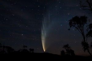
Its perihelion is 0.17 Astronomical Units (AU), where one AU is the distance of the earth from the sun, or about 149,597,871 km. This means it came as close as 25,544,000 km to earth. However, with an eccentricity of 1.000019, its aphelion is about 4100 AU and it has a period of about 92,600 years! Although we know its last perihelion was in 2007, it is unknown when it will return, or even where humans may be settled in our galaxy that far in the future.
In the next section, we will consider hyperbolic orbits. But first, work through this example problem to see how well you understand the concepts from this section. The answers and solutions are at the end of this chapter.
EXAMPLE 3
A Jupiter probe is in a circular orbit around Earth with a radius of 25,000 km. The next step on the way to Jupiter is to thrust so the probe can enter into an escape orbit.
-
- Determine the probe’s velocity in this circular orbit.
- Determine the minimum velocity required to enter a parabolic trajectory at that radius.
- Determine the difference in the specific kinetic, potential, and mechanical energies between the two orbits.
HYPERBOLIC ORBITS
Hyperbolic orbits, as seen in Figure 12, are very useful, especially for interplanetary travel. An interplanetary probe must have some speed left over after it escapes the earth’s gravitational field.
The semi-major axis of a hyperbolic orbit is negative. This seems like a strange phenomenon, but it makes sense if you consider the specific mechanical energy of a hyperbolic orbit:
(19)
[latex]\large \varepsilon = -\frac{\mu}{2a}[/latex]
If the semi-major axis, a, is negative, this will make the specific mechanical energy positive. Thus in the energy equation,
(20)
[latex]\large \varepsilon = \frac{V^2}{2}-\frac{\mu}{R}[/latex]
as R gets very large, the potential energy term gets smaller and smaller, leaving only kinetic energy!
In addition, the eccentricity of a hyperbolic orbit is greater than one. The eccentricity gets larger the more spread out the arms are. For some examples of how eccentricity is affected based on the shape of the hyperbola, see Figure 13 below. For more details on hyperbolic orbit geometry, see Bate.
Also, a similar form to find radius of perigee for a parabolic orbit is used, while radius to apogee is infinitely large.
(21)
[latex]\large R_{p}=\frac{p}{2}[/latex]
So now let’s consider how hyperbolic trajectories are used for interplanetary travel and some terminology associated with them. If you give a spacecraft the exact escape speed, it will just barely escape the gravitational field. This means that its speed will approach zero as its distance from the earth approaches infinity. However, if we give our spacecraft more than the escape speed at a point near the earth, as visualized in Figure 14, the speed at a great distance from the earth will have some positive value. This residual speed that the spacecraft would have left over is called the “hyperbolic excess speed,” or [latex]V_{\infty}[/latex].
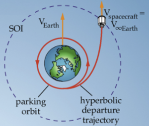
If a satellite starts in a parking orbit near earth, we can find the speed needed to depart from the parking orbit to achieve [latex]V_{\infty}[/latex] at an infinite distance from the earth, which we will consider the earth’s Sphere of Influence, or SOI. Although it is difficult to find an agreed-upon definition, for our purposes we can consider it approximately 1.5 million km from the earth.
We can then calculate the boost needed to get on the hyperbolic departure trajectory to the edge of the earth’s SOI by writing the energy equation at two points on this orbit. The first point is at the parking orbit, called Burnout Velocity, [latex]V_{BO}[/latex]. The second point will be at the edge of the earth’s SOI, or [latex]V_{\infty}[/latex]. Since:
(22)
[latex]\large \varepsilon = \frac{V^2}{2}-\frac{\mu}{R}[/latex]
Since the energy needed at the edge of the earth’s SOI, or
(23)
[latex]\large \varepsilon_{\infty}=\frac{V^2_{\infty}}{2}-\frac{\mu}{R_{\infty}}=\frac{V^2_{\infty}}{2}[/latex]
This energy must be equal to the energy needed to get on the hyperbolic escape trajectory at the parking orbit, or
(24)
[latex]\large \varepsilon_{h} = \frac{V^2_{BO}}{2}-\frac{\mu}{R_{BO}}[/latex]
So
(25)
[latex]\large \frac{V^2_{BO}}{2}-\frac{\mu}{R_{BO}} = \frac{V^2_{\infty}}{2}[/latex]
Rearranging this equation yields:
(26)
[latex]\large V^2_{BO}=V^2_{\infty} + \frac{2\mu}{R_{BO}}[/latex]
Notice the last term:
(27)
[latex]\large \frac{2\mu}{R_{BO}} = V^2_{esc}[/latex]
So our final equation relating these velocities become:
(28)
[latex]\large V^2_{BO}=V^2_{\infty} + V^2_{esc}[/latex]
Now let us recap the meaning of these velocity terms.
[latex]V_{BO} =[/latex] the velocity needed at the parking orbit to achieve the velocity needed at the edge of the Earth’s SOI
[latex]V_{\infty} =[/latex] the velocity needed at the edge of the Earth’s SOI to break away from the earth’s influence
[latex]V_{esc} =[/latex] the velocity need to barely get to the Earth’s SOI with no excess velocity
Finally, to get from an initial parking orbit (assuming circular) to a hyperbolic escape orbit, we must first know the spacecraft’s velocity in the parking orbit:
(29)
[latex]\large V_{Park} = \sqrt{\frac{\mu}{R_{Park}}}[/latex]
Then
(30)
[latex]\large V_{BO} = \sqrt{V^2_{\infty}+V^2_{esc}}[/latex]
So the change in velocity, or boost needed to escape the earth’s sphere of influence, is given by:
(31)
[latex]\large \Delta V_{needed}=|V_{BO}-V_{Park}|[/latex]
Where the vertical lines represent the absolute value of the result.
Although we do not encounter hyperbolic trajectories much on the earth or for the earth-orbiting satellites, they are very common in interplanetary travel and among bodies in our solar system. Meteors that strike the earth travel on hyperbolic paths relative to the earth. The Perseids Meteor Showers shown in Figure 16 are one example. These meteors, which peak during mid-August, originate from comet 109P/Swift-Tuttle (Figure 15). Swift-Tuttle is in an elliptical orbit around the sun and has a period of 133 years. Comet Swift-Tuttle last visited the inner solar system in 1992. When it came around the sun, it left a dusty trail behind it. Every year the earth passes through these debris trails, bits of leftover comet particles collide with our atmosphere and disintegrate, creating fiery and colorful streaks in the sky. At its peak, it can result in up to 100 meteors per hour at speeds of approximately 59 km/s (NASA 2019).

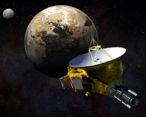
Interplanetary missions must use hyperbolic trajectories that are relative to the earth if we want the interplanetary probe to break away from the earth’s gravitational field. An interesting interplanetary spacecraft is New Horizons, visualized in Figure 17, which was sent to explore far into our solar system. By the time it reached Pluto, the spacecraft had travelled farther away and for a longer time period, more than nine years, than any previous deep space spacecraft ever launched. It observed Pluto close up, flying by the dwarf planet and its moons in July 2015 (NASA 2020).
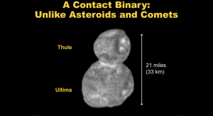
In early 2019, New Horizons flew past its second major science target, 2014 MU69, the most distance object ever explored up close. New Horizons discovered the object is a contact binary, two different spherical objects (Figure 18). The lobes were formed separately and then eased together over four billion years ago at speeds between one to two miles per hour. These two rocks were then pulled together by the extremely weak gravitational forces of each other, nudging together at such slow speeds that initial observations from New Horizons do not reveal any stress fractures or damage from the ‘collision.’ More discoveries by New Horizons are yet to come (Gebhart, 2019).
In order to get on this interplanetary trajectory, New Horizons was launched in January 2006 from Cape Canaveral Air Force Station. (You will learn later in this book why the Cape is an ideal location from which to launch an interplanetary probe). It was launched into a hyperbolic departure trajectory, which took it on a path by Jupiter. The giant planet’s gravitational pull helped it “slingshot” the spacecraft toward the outer solar system.
There are two reasons why the New Horizons science team wanted to reach Pluto as soon as possible. The first had to do with Pluto’s atmosphere. Since 1989, Pluto has been moving farther from the Sun, getting less heat every year. As Pluto gets colder, scientists expect its atmosphere will “freeze out,” so the team wanted to arrive while there was a chance to study a thicker atmosphere.
The second reason was to map as much of Pluto and its largest moon, Charon, as possible. On the earth, the North Pole and other areas above the Arctic Circle have half a year of night and half a year of daylight. In the same way, parts of Pluto and Charon never see the Sun for decades at a time. The longer the wait, the more of Pluto and Charon would have been shadowed in a long “arctic night,” impeding the spacecraft’s ability to take pictures of the surface in reflected sunlight.
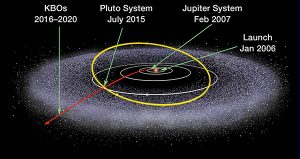
In February 2007, New Horizons passed through the Jupiter system at more than 50,000 mph, ending up on a path that got it to Pluto on July 14, 2015, about nine and a half years later, compared to the 30 years or so it would take to get there directly. Figure 19 shows the path New Horizons took to get to Jupiter and the Kuiper Belt Objects (KBOs). You will learn about gravitational assist trajectories later. Without the use of hyperbolic trajectories, however, New Horizons would have never left the earth’s gravitational field at all!
Now, work through this example problem to see how well you understand the concepts from this section. The answers and solutions are at the end of this chapter.
EXAMPLE 4
A spacecraft is launched from a parking orbit around earth to Mars.
Given:
[latex]\large V_{\infty} = 2.94 km/s[/latex]
[latex]\large R_{Park\_at\_Earth} = 6697[/latex] (circular)
Find:
a) [latex]\varepsilon_{\infty}[/latex] energy needed at the edge of the Earth’s sphere of influence
b) [latex]V_{BO} =[/latex] the velocity needed at the parking orbit to achieve the velocity needed at the edge of the Earth’s SOI
c) [latex]\Delta V_{needed} =[/latex] The boost needed to get the spacecraft from its parking orbit onto the hyperbolic departure trajectory
SUMMARY
In this chapter, we first discussed how a satellite gets into orbit and related it to the conic sections. We then reviewed elliptical orbits and its parameters, then extended these results to consider the other conic sections. Below is a summary of the orbits types and the value, or range of values, for some of their orbital parameters.
| Orbit Type | Semi-major axis, [latex]a[/latex] | eccentricity, [latex]e[/latex] | Specific mechanical energy, [latex]\varepsilon[/latex] |
| Ellipse | [latex]a > 6578 km[/latex]* | [latex]0 < e < 1[/latex] | [latex]\varepsilon < 0[/latex] |
| Circle | [latex]a = R[/latex] (constant) | [latex]e = 0[/latex] | [latex]\varepsilon < 0[/latex] |
| Parabola | [latex]a = \infty[/latex] | [latex]e = 1[/latex] | [latex]\varepsilon = 0[/latex] |
| Hyperbola | [latex]a < 0[/latex] | [latex]e > 1[/latex] | [latex]\varepsilon > 0[/latex] |
* Earth’s radius + 200 km
Check your understanding with this quick quiz!
SOLUTIONS TO EXAMPLES:
***Example 1 Solution***
The altitude of a satellite at perigee is 500 km and its orbital eccentricity is 0.1. Find:
a) The satellite’s altitude at apogee
Since
[latex]\large R_{p}=a(1-e)[/latex]
[latex]\large 6378[/latex] km [latex]+[/latex] [latex]500[/latex] km [latex]= a(1-0.1)[/latex]
[latex]\large a = 6878/0.9[/latex] km
[latex]\large a = 7642[/latex] km
and
[latex]\large R_{a} = a(1+e) = 7642(1+0.1)[/latex]
[latex]\large Ra = 8406 km[/latex]
So the satellite’s altitude at apogee [latex]= 8406 - 6378[/latex] km
Altitude at apogee = 2028 km
b) The orbit’s specific mechanical energy, [latex]\varepsilon[/latex]
Since
[latex]\large \varepsilon = -\frac{\mu}{2a}[/latex]
[latex]\large \varepsilon = -\frac{398600.5\,\frac{km^3}{s^2}}{2(42241\,km)} = -4.718\,\frac{km^2}{s^2}[/latex]
so
[latex]\large \varepsilon =[/latex] -26.08 km2/s2
c) The magnitude of the orbit’s specific angular momentum, h
Since
[latex]\large h=\sqrt{\mu a(1-e^2)}[/latex]
[latex]\large h=\sqrt{398600.5*7642*(1-0.1^2)}[/latex]
so
h = 54915 km2/s
d) The satellite’s speed at apogee
Since
[latex]\Large h = R_{a}V_{a}[/latex]
[latex]\Large V_{a} = \frac{h}{R_{a}}[/latex]
so
Va = 6.53 km/s
***Example 2 Solution***
A geostationary orbit, GEO, is one in which a satellite always remains above the same point on the earth’s equator. For a GEO satellite, the radial from the center of the earth to the satellite must have the same angular velocity as the earth itself, or a period of 24 hours.
a) Calculate the altitude of a GEO orbit.
Since
[latex]\large Period = 2 \pi \sqrt{\frac{a^3}{\mu}}=24\:hours[/latex]
So
[latex]\large a=\sqrt[3]{ \left( \frac{24 \, \times \, 3600 \frac{sec}{hr}}{2\pi} \right) ^2 \, (398600.5 \, \frac{km^3}{s^2})}[/latex]
[latex]\large a = 42241[/latex] km
altitude of a GEO satellite = 35,863 km
b) Calculate the specific mechanical energy, [latex]\varepsilon[/latex], of a GEO satellite’s orbit.
[latex]\large \varepsilon = -\frac{\mu}{2a}[/latex]
[latex]\large \varepsilon = - \frac{398600.5\:\frac{km^3}{s^2}}{2(42241\:km)}[/latex]
[latex]\large \varepsilon[/latex] = -4.718 km3/s2
c) Calculate the speed of a GEO satellite.
[latex]\large V = \sqrt{\frac{\mu}{R}}[/latex]
[latex]\large V = \sqrt{\frac{398600.5\:\frac{km^3}{s^2}}{42241\:km}}[/latex]
so
V = 3.07 km/s
***Example 3 Solution***
A Jupiter probe is in a circular orbit around the earth with a radius of 25,000 km. The next step on the way to Jupiter is to thrust so the probe can enter into an escape orbit.
- Determine the probe’s velocity in this circular orbit.
Since
[latex]\large R = 25,000 \, km[/latex]
[latex]\large V = \frac{\mu}{R}=\sqrt{\frac{398600.5\:\frac{km^3}{s^2}}{25000\:km}}[/latex]
So
V = 3.99 km/s
2. Determine the minimum velocity required to enter a parabolic trajectory at that radius.
[latex]\large V_{esc} = \sqrt{\frac{2\mu}{R}}=\sqrt{\frac{2(398600.5\:\frac{km^3}{s^2})}{25000\:km}}[/latex]
So
V = 5.65 km/s
3. Determine the difference in the specific kinetic, potential, and mechanical energies between the two orbits.
Orbit 1 (circular parking orbit)
[latex]\large KE = \frac{V^2}{2}=\frac{3.99^2}{2}=7.96\:\frac{km^2}{s^2}[/latex]
[latex]\large PE = -\frac{\mu}{R} = - \frac{398600.5\frac{km^3}{s^2}}{25000\:km} = -15.94\:\frac{km^2}{s^2}[/latex]
[latex]\large \varepsilon[/latex] = -7.98 km2/s2
Orbit 2 (Escape Orbit)
[latex]\large KE = \frac{V^2}{2}=\frac{5.65}{2}=15.96\:\frac{km^2}{s^2}[/latex]
[latex]\large PE = -15.96\:\frac{km^2}{s^2}[/latex]
[latex]\large \varepsilon = 0[/latex]
So PE doesn’t change (any small difference is due to round-off error) while [latex]KE[/latex] changes by [latex]8\;km^2/s^2[/latex].
Since the Specific Mechanical Energy changes by approximately [latex]8\;km^2/s^2[/latex], all of the energy added is strictly due to the change in [latex]KE[/latex].
***Example 4 Solution***
A spacecraft is launched from a parking orbit around earth to Mars.
Given:
[latex]\large R_{Park\_at\_Earth} = 6697[/latex] (circular)
Find:
a) [latex]\large \varepsilon_{\infty}[/latex] energy needed at the edge of the Earth’s sphere of influence
[latex]\large \varepsilon_{\infty} = \frac{V^2_{\infty}}{2} = 0.5 * (2.94\:km/s)^2[/latex]
[latex]\large \varepsilon_{\infty}[/latex] = 4.32 km2/s2
b) [latex]V_{BO}=[/latex]the velocity needed at the parking orbit to achieve the velocity needed at the edge of the Earth’s SOI
[latex]\bf{V^2_{BO} = V^2_{\infty}+V^2_{esc}}[/latex]
So
[latex]\large V_{BO} = \sqrt{(2.94)^2+\frac{2\,*\,398600.5\:\frac{km^3}{s^2}}{6697\:km}}[/latex]
[latex]\large V_{BO} = 11.3\:km/s[/latex]
c) [latex]\Delta V_{needed} = |V_{BO}-V_{park}| =[/latex] The boost needed to get the spacecraft from its parking orbit onto the hyperbolic departure trajectory
The satellite’s velocity in its original parking orbit is
[latex]\large V = \sqrt{\frac{\mu}{R}}[/latex]
so
[latex]\large V_{Park} = \sqrt{\frac{398600.5\:\frac{km^3}{s^2}}{6697\:km}}[/latex]
[latex]\large V_{Park}=7.71\:km/s[/latex]
and
[latex]\large \Delta V_{needed} = |11.3-7.715|\:km/s[/latex]
So
[latex]\large \Delta V_{needed}[/latex] = 3.585 km/s
REFERENCES
American Mathematical Society. (2005). Sling Shots and Space Shots. http://www.ams.org/publicoutreach/feature-column/fcarc-slingshot.
Ashish. Why do rockets follow a curved path instead of going straight into space? (2021, 3 February). https://www.scienceabc.com/nature/universe/why-do-rockets-follow-a-curved-trajectory-while-going-into-space.html
Bate, R. R., Mueller, D. D., White, J. E., & Saylor, W. W. (1971). Fundamentals of astrodynamics. Mineola (N.Y.): Dover Publications.
Britannica. Orbit. (2021). https://www.britannica.com/science/orbit-astronomy
European Space Agency navipedia. (2020, 20 November). GPS Space Segment. https://gssc.esa.int/navipedia/index.php/GPS_Space_Segment
Gebhardt, W. (2019, January 02). 2014 MU69 Revealed as a Contact Binary in First New Horizons Data Returns. https://www.nasaspaceflight.com/2019/01/2014-mu69-contact-binary-first-new-horizons-returns/
NASA Solar System Exploration. (2019, 19 December). Perseids: In Depth. https://solarsystem.nasa.gov/asteroids-comets-and-meteors/meteors-and-meteorites/perseids/in-depth/
NASA Solar System Exploration. (2020, 7 October). New Horizons: In Depth. https://solarsystem.nasa.gov/missions/new-horizons/in-depth7
The Physics Classroom. What is a projectile? (n.d.) https://www.physicsclassroom.com/Class/vectors/
Schroeder, Daniel V. Newton’s cannon (2020, 20 January). https://physics.weber.edu/schroeder/software/NewtonsCannon.html
Sellers, Jerry Jon. (2005). Understanding Space: An Introduction to Astronautics, 3rd edition. McGraw-Hill.
Media Attributions
- Figure 1: Newton’s Cannon HTML5 Simulator © Michael Fowler is licensed under a Public Domain license
- Figure 2: Newton’s Cannon HTML5 Simulation Screenshot © Fowler and Dolgert is licensed under a Public Domain license
- Figure 3: Rocket Launch in Space DIAGRAM1 © Arjit Raj is licensed under a Public Domain license
- Figure 23: Two-Body EOM Geometry (Edited) © John Siegenthaler is licensed under a Public Domain license
- Figure 5: Earth’s Orbit © Encyclopædia Britannica Inc. is licensed under a CC0 (Creative Commons Zero) license
- Figure 6: Molniya Orbit © Shajind is licensed under a Public Domain license
- Figure 7: Satellite’s Orbits (Edited) © NASA is licensed under a Public Domain license
- Figure 8: GPS Constellation © Jose Caro is licensed under a Public Domain license
- Figure 9: Azimuthal Equidistant Projection (Edited) © Janosch Gaia is licensed under a Public Domain license
- Figure 10: Parabolic Orbit © Brandir is licensed under a CC BY-SA (Attribution ShareAlike) license
- Figure 11: Comet P1 McNaught02 © fir0002 is licensed under a CC BY-NC (Attribution NonCommercial) license
- Figure 12: Hyperbolic Orbit © Brandir is licensed under a CC BY-SA (Attribution ShareAlike) license
- Figure 13: Hyperbolas © Bill Casselman is licensed under a CC0 (Creative Commons Zero) license
- Figure 14: Hyperbolic Departure © Lynanne George is licensed under a Public Domain license
- Figure 15: Comet Swift-Tuttle © Takoda Edlund is licensed under a Public Domain license
- Figure 16: Perseid Meteor Shower © Lindsay Brooke is licensed under a Public Domain license
- Figure 17: A New Horizons Pluto Flyby (Artist Concept) © Johns Hopkins is licensed under a Public Domain license
- Figure 18: A Contact Binary: 2014 MU69 © NASA/AP is licensed under a Public Domain license
- Figure 19: Kuiper Belt: In Depth (Edited) © NASA is licensed under a Public Domain license
