TIME

It might be said a lot, but time is truly of the essence. It is often considered a fourth dimension and is not only used in all fields of science, but is also crucial. Astrodynamics and orbital mechanics is no exception. Objects in space move at such high speeds that it is crucial to have a way to describe the time that is passing by in a precise way. It also needs to be noted that we track objects in space over incredibly long periods of time. Therefore, we need a time interval that is also repeatable. This chapter will begin by introducing how and why we have defined time in the way that most are probably familiar with, solar time, and how we are going to redefine it, sidereal time. Understanding how we define time will be important in the next section when we discuss launch windows and beyond.

SOLAR TIME

Time as most people know it is broken down into seconds, minutes, hours, days, etc. This goes back to when time was first established with the location of the Sun. As you may know, a day is when the Earth makes one rotation around its axis. A day was initially and roughly defined by observing the shadows on a sun dial. This device, pictured below, used the angle of the shadow produced by the gnomon, arm, to determine how many hours have passed in the day. It was marked when the Sun would continually pass the same point every day. It was unrefined as the people at the time didn’t have a more accurate or precise way to measure, but it still gave the first definition to a day. This is called an apparent solar day.

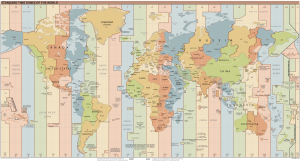
For almost every place on earth, the time 1200, otherwise known as 12:00 PM, is defined as when the Sun is positioned directly upwards. So, with different parts of the world having that occurrence at different times throughout the day, how do we compensate? The answer is time zones. The world has 24 distinct time zones that are positioned 15° of longitude apart from each other. As seen in the figure below, most countries do not fit into their respective time zones perfectly, and some use slight variations of this method, such as being on half-hour intervals, but as seen, most follow the 15° rule. With this, it should be noted that the Earth’s orbit around the Sun has a slight eccentricity of e=0.017 and is therefore not perfectly circular. Also, the Earth’s axis is not perpendicular to the plane of orbit. Because of these facts, there is a slight variation to the apparent solar day throughout the year. This is bad for us as we want everything to be accurate and precise. To make up for this, a mean solar day is calculated by taking the average of apparent solar days in a year. To do this, we make the assumption that the Earth’s orbit is perfectly circular and split it into 365 days. Measuring time in reference to this day is known as mean solar time. This is the day and time that almost all people follow and is shown on the clocks we use.

*Fun Fact: There are a total of 38 local time zones currently used throughout the world when taking into consideration half and quarter time intervals, daylight savings, and the International Date Line.

Again, there arises a problem. What time zone do we use universally if it is a different time in more than 24 places at any given instant? The answer lies within Greenwich, England. This city houses The Royal Observatory which was constructed in 1675 and is used to track the movement of the Moon and location of the stars. What is also special about Greenwich is it just so happens to lie on the Prime Meridian, which is defined by its 0° longitude. We use this time zone to be the universal time. Using the mean solar time, we rather literally call this time zone Greenwich Mean Time, or GMT. It is also referred to as Universal Time, UT, as well as Zulu, Z, time.

As it pertains to astrodynamics, and more specifically launch windows, there is one more piece of information that was ignored in everything talked about previously. This is the fact that this way of telling time is not inertial. When we previously defined the orbital elements, we defined them with respect to the geocentric-equatorial coordinate system, otherwise known as coordinate frame. With this being an Earth-centric coordinate system, the Sun, and therefore our solar time references, seem to move with respect to the solar system and Earth orbits around it. To deal with this issue, we will identify a new way to describe time: sidereal time.

SIDEREAL TIME

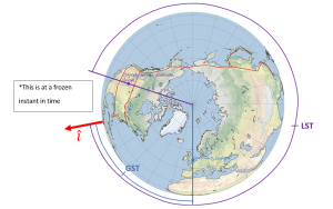
Sidereal time, unlike solar time, is inertial and is measured as the angle between a given longitude line and the vernal equinox. Similarly, a sidereal day is established as a specific longitude continuously passing the vernal equinox after a full rotation of the Earth. Remember that the [latex]\hat{I}[/latex] vector points towards the vernal equinox so it can be thought of that sidereal time is measured from the [latex]\hat{I}[/latex] vector. The vernal equinox is chosen because, as opposed to the Sun, which is approximately 150 million km away from the earth, it is measured relative to far away constellations, for which none lie less than 100 lightyears away. Much like solar time, there is a universal longitude. This is again a longitude of 0° and the time associated with this longitude is defined as Greenwich Sidereal Time, GST. The sidereal time at any given longitude can also be found and is defined as Local Sidereal Time, LST. These are the two ways to define time that will be seen throughout nearly the rest of the course. The difference between these two can be seen in the image below.

Learning how to talk and write about time in degrees, as well as go between hours and degrees, is crucial. It is quite simple to go between the two. If the earth rotates 360° in 24 hours, then it can be reduced down to say that it rotates 15°/hr (ω_Earth). This is the reason time zones are split into 15° intervals. With this relationship, time can be easily converted between degrees and hours as seen in the equation below.

Time (degrees) = Time (hours) * 15°/hr

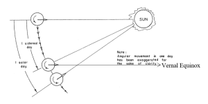
The big question is: where do we see the big differences between mean solar days and sidereal days? Why not just use mean solar days and split it up into degrees. Well, because of the aforementioned inertial reference point, a mean solar day is actually approximately 4 minutes longer than a sidereal day. This is because the Earth rotates just a little more than 360° in order to bring the sun back to its observed spot. This is caused because the Sun is actually moving and changing its position slightly. On the other hand, the vernal equinox is so incredibly far away, it is essentially stationary from our point of view, therefore one full rotation of the Earth in reference to it is simply 360°. A largely overstated view of these times can be observed under the relationship seen further down. Though it should be noted that translating between mean solar time and sidereal time is not as easy as adding 4 minutes; it requires the knowledge of the vernal equinox at some previous date, and with some propagation, it can be found. For the purposes of this course and book, that knowledge is not needed.

23 hours 56 minutes 4 seconds mean solar time = 24 hours sidereal time

Note if you are given GST,

Now, before we move onto launch windows, take this short quiz to test your understanding on time.

LAUNCH WINDOWS

A large part of orbital mechanics is actually getting the object we want into space. Most of the time, we have a specific set of orbital elements (COE’s) that are predefined, and our job is to get that object into that orbit. A launch window is a period of time that we have where we can directly send the object into the specific obit we want. It would be possible to simply shoot it to an arbitrary location and do some orbital maneuvers that we will discuss later, but that would be a waste of fuel and time. Instead, we can determine a set launch time and angle that will essentially place our object directly into orbit. Unfortunately, there are some limitations such as launch site, as well as the limitations of the launch vehicle that could cause a direct launch to be impossible.

There are 3 cases that need to be considered: when inclination is less than the launch site latitude, when inclination is equal to the launch site latitude, and when inclination is greater than the launch site latitude. This will take getting to know some knew terms. We will look at these terms morse closely later, but it is good to be familiar with the nomenclature.

L₀ : Launch Site Latitude

LWST: Launch-Window Sidereal Time

γ: Launch-Direction Auxiliary Angle

α: Inclination Auxiliary Angle

δ: Launch-Window Location Angle

β: Launch Azimuth

In order to determine when to launch, we must use the new local sidereal time we learned. We define the LST when the launch site is in position of launch-window sidereal time, LWST. “In position” is defined as one of the intersections of the launch site and the orbital plane. When the LST is equal to the LWST, it is time to launch.

CASE 1: i < L₀

The first case we are going to look at is the case where the inclination is less than the launch site latitude. This first case is quite simple because there is no way to launch the object directly into orbit. There would not be time when the launch site would intersect with the inclination. It would require a launch into an inclination of the same latitude with a plane change to reach its desired inclination.

CASE 2: i = L₀

When it comes to launch windows that do exist, there are two types of orbits: direct and indirect (retrograde). Respectively, they exist when the launch site latitude is less than or equal to the inclination (L₀[latex]\le[/latex]i) for direct orbits, or when launch site latitude is less than or equal to 180° minus the inclination (L₀[latex]\le[/latex]180º-i) for in-direct/retrograde orbits.

The second case is when the inclination has the same angle as the latitude of the launch site. In this case, there is only one singular time when the launch site intersects with the inclination plane. Therefore, there is only one launch window. This specific time will occur only at the most northern end of the orbital plane. This is shown best in the model below.

For this case, note that in the model above this intersection is found 90° from the ascending node. As a reminder, the ascending node is when an object in orbit passes from the southern hemisphere to the northern hemisphere. This makes finding the LWST not very difficult with the help of the right ascension of the ascending node (RAAN, Ω). If we put all of this together we will find that:

LWST = Ω + 90°

CASE 3: i > L₀

There remains one last case for launch-windows and this is if the inclination is greater than the launch site latitude. In this case, there happens to be two launch windows per day. In its inertial space, the orbital plane stays fixed. This results in two intersections when the rotation of the Earth brings the launch site under said orbital plane. Both windows can be seen in the following model. We define both of these by which one is nearest to either the ascending or descending node. Remember that the ascending node is where the object in orbit passes from the southern hemisphere to the northern and similarly, the descending node is where the object in orbit passes from the northern hemisphere to the southern. In the figure below, we see the first opportunity is the ascending-node opportunity and the second opportunity is the descending-node opportunity.

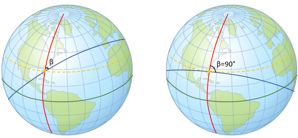
With Case 3 being more complicated than the first two cases, we need to take a look at some 3-dimensional geometry. There are three lines that need to be drawn to define the spherical circle we will use. The first line is the ground track for the orbit. We will speak more of the ground tracks in the next chapter, but right now, it just needs to be thought of as the path of the orbit traced on the Earth. The second line is the line of the equator. The third line that needs to be drawn is the local longitude of the launch site. When these are drawn as seen in the graphic below, with the yellow dot representing the launch site (using Cape Canaveral in this example), a right spherical triangle appears. This special type of triangle is different than a planar triangle as the sum of the angles is greater than 180°.

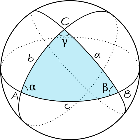
Note that with spherical triangles, the three sides of the triangle are measured as angles. They are measured from the center of the sphere; even though the Earth is not perfectly spherical, it is assumed so for the purposes of this geometry calculation. In order to find the variables we are looking for, we need to use the spherical version of the law of cosines which is stated as:

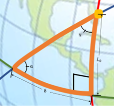
The variables we are defining with the triangle we created are the inclination auxiliary variable, α, the launch-direction auxiliary variable, γ, the launch-window location angle, δ, and the launch site latitude, L₀. We define the inclination auxiliary variable, α, as the ascending node between the equator and the orbit. Note that for direct orbits, α is equal to our inclination, i. The launch-direction auxiliary variable, γ, is measured between the longitudinal line and the orbital ground track. The launch-window location angle, δ, is measured on our triangle following the equator. This is the angle that becomes most important to us and will lead to a direct substitution to find the LWST. These variables can be seen pictorially in the following zoomed in picture of the triangle we created.

Now, let us use the second spherical law of cosines in order to determine α:

Simplifying down with cos(90°) = 0 and sin(90°) = 1, this equation reduces down to:

Rearranging for γ, we get:

Using spherical geometry again, we find that:

Simplifying down with cos(90°) = 0 and sin(90°) = 1, this equation reduces down to:

Rearranging for δ, we get:

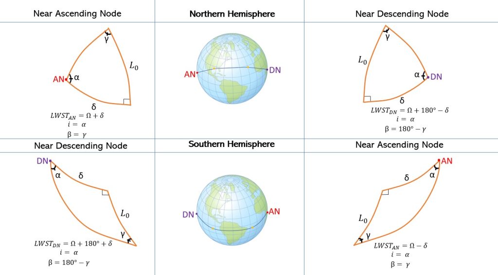
For a direct orbit in the Northern Hemisphere, we can now use the following equation to determine the LWST at the ascending node:

LWST_AN  = Ω + δ

As well as at the descending node:

LWST_DN  = Ω + (180º – δ)

There is one final angle that is important to be considered when it comes to launch windows, and that is the launch azimuth, β. This angle is so important because it tells us which direction to launch in. One big assumption in determining this angle is considering the Earth to be non-rotating. To measure this value, we start at the launch site, go directly north, and measure going clockwise. This is the angle between that “upwards” direction and the launch direction. This can be seen more clearly in the image below.

A good way to think about this angle is that it is measured exactly like it would appear on a compass. This is to say that if the launch azimuth was directly north, it would be measured as 0°, directly south would be measured as 180°, east=90°, and west=270°.

As you can see in the figure above, β is equal to γ for this ascending-node opportunity in a Northern Hemisphere site. Similarly, for a descending-node opportunity from a Northern Hemisphere site, β = 180° – γ. For sites in the Southern Hemisphere, these equations stay the same. Therefore, for whichever hemisphere, the launch azimuth can be found using the following equations:

Ascending-node opportunity: β = γ

Descending-node opportunity: β = 180° – γ

Example 1

Given the following satellite and launch site parameters:

LST = 3 hours

L₀ = 32°

RAAN = 105°

i = 55°

Find the launch window sidereal time in hours soonest to the current time, as well as its respective launch azimuth, β.

With launch sites in the southern hemisphere, not much changes besides the spherical triangle getting turned 180° as well as what is defined as the ascending node and the descending node. Remember that the ascending node is defined as when an object in orbit passes from the Southern Hemisphere to the Northern Hemisphere, and vice-versa for the descending node. That means that these two nodes are “flipped” if the site is in the Northern Hemisphere versus the Southern Hemisphere. So, don’t think of the nodes as the “left” or “right” nodes on the globe. Think about how the object is traveling. If you do, the process will be just the same as detailed in the small summary below:

Prograde Orbits

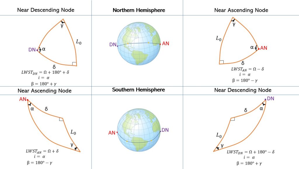
Up to this point, everything talked about has been about direct (prograde) orbits, though it is important to deal with retrograde orbits as well. When doing this, it is very important to draw the pictures out carefully and understand where everything we are getting is coming from. Though, we will follow nearly the same exact process to give us the result of:

Retrograde Orbits

]Take this short quiz to test your understanding of this chapter.

SOLUTIONS TO EXAMPLES:

***Example 1 Solution***

Given the following satellite and launch site parameters:

LST = 3 hours

L₀ = 32°

RAAN = 105°

i = 55°

Find the launch window sidereal time in hours soonest to the current time as well as its respective launch azimuth, β.

Solution:

The inclination is greater than the launch site latitude, therefore this is a Case 3. Also notice that the orbit is direct with the inclination being less than 90°. Therefore:

α = i = 55°

With the current LST of 3 hours, the ascending-node opportunity at 8.73 hours is soonest, so that is when we will decide to launch.

REFERENCES

Bate, R. R., Mueller, D. D., &amp; White, J. E. (2015). Fundamentals of astrodynamics. Dover Publications.

Expanded world time zone map. Large World Time Zone Map. https://www.timetemperature.com/time-zone-maps/large-world-time-zone-map.shtml

Animation of rotating Earth at night.webm. Wikimedia Commons. https://commons.wikimedia.org/wiki/File:Animation_of_Rotating_Earth_at_Night.webm

How many time zones are there? How Many Time Zones in the World. https://www.timeanddate.com/time/current-number-time-zones.html

Projects, C. to W. (2020, November 12). North Pole. Wikimedia Commons.  https://commons.wikimedia.org/wiki/North_Pole

Sellers, J. J., Astore, W. J., Giffen, R. B., &amp; Larson, W. J. Understanding Space An Introduction to Astronautics (3rd ed.). The McGraw-Hill Companies, Inc.

Simple graphic illustration globe showing latitude stock vector (royalty free). Shutterstock. https://www.shutterstock.com/image-vector/simple-graphic-illustration-globe-showing-latitude-13234843

Spherical cosine law. Mathematics@CUHK. (2010, November 8).  https://cuhkmath.wordpress.com/2010/10/04/spherical-cosine-law/

Staff, F. A., &amp; Farmers’ Almanac Staff https://www.farmersalmanac.com/author/fa-admin. (2022, July 5). Sundials: Where Time began. Farmers’ Almanac – Plan Your Day. Grow Your Life. November 7, 2022, from https://www.farmersalmanac.com/sundials-time-began-18870

Sun PNG images. Free Icons PNG. https://www.freeiconspng.com/images/sun

Unsplash.. Download Free Pictures &amp; Images [HD]. Unsplash. https://unsplash.com/images

Vallado, D. A., & McClain, W. D. (2013). Fundamentals of Astrodynamics and Applications. Microcosm Press.