8 Chapter 8 – Rendezvous

In this chapter, we will consider another type of maneuver called a Rendezvous maneuver. Have you ever thought about how we move one object to another in orbit? We cannot exactly move in a straight shot from one location to another. That would take way too much fuel and we would end up in a different orbit. Like the other maneuvers, we are going to work with orbital mechanics to make it as fuel efficient as possible.

You might wonder why we are interested in Rendezvous maneuvers. This specific type of maneuver is used in many applications. For example, the International Space Station needs to be resupplied. If we launch supplies toward the ISS, how do we know the station will be there when the supplies arrive at its orbit? A carefully planned Rendezvous maneuver! We may also have to refuel and make repairs on objects in orbit, such as the repair mission performed on the Hubble Telescope (NASA, 2020). This maneuver is also used for space junk cleanup and even interplanetary missions. Thus, this type of maneuver is very important in Astrodynamics.

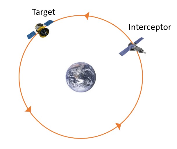
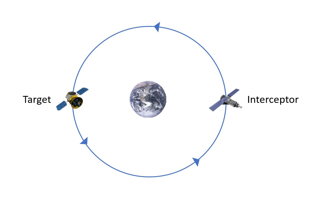
Let us begin by defining the two main bodies in a Rendezvous problem: the target and the interceptor. The target is going to be the satellite that remains untouched. It will stay in its same orbit, and as the name suggests, will be the target that the other satellite is aiming for. That other body is the interceptor. The interceptor is the satellite that will have its orbit manipulated. Its goal is to be in the same orbit at the same location as the target. The following image will be different for every situation we consider, but it gives a general look at an interceptor and a target to show how we will model them in this chapter.

CO-PLANAR

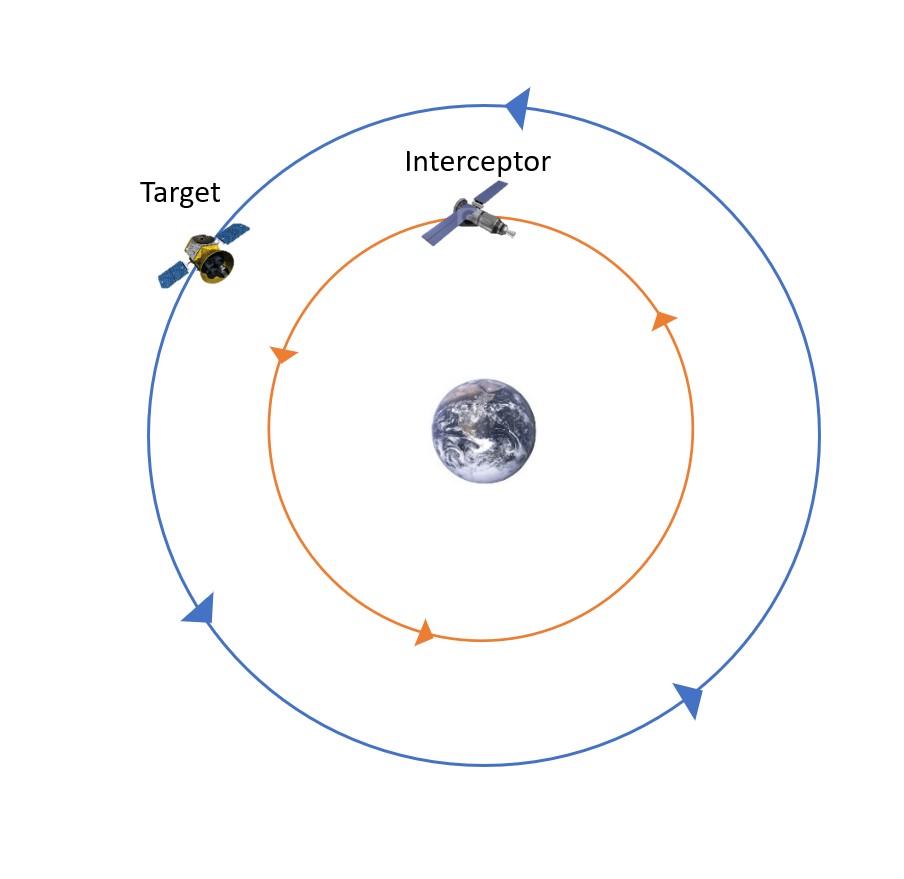
The first kind of Rendezvous maneuver we are going to discuss is a co-planar rendezvous. In this situation, the target and interceptor occupy distinct orbits, yet they are co-planar, as seen below:

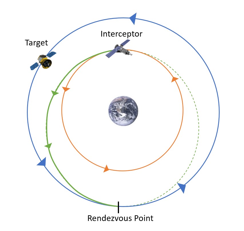
In the big picture, we are moving the interceptor from a smaller orbit to a larger orbit. If we think about the most efficient way we know to do this, the idea of a Hohmann Transfer comes up. This is exactly what is going to be used to complete this maneuver. However, since we cannot just have it at any given location in the final orbit, then we need to carefully consider the timing of both the interceptor’s maneuver, as well as the timing of the target satellite’s position. To do this, we want to plan for both of them to meet at the Rendezvous Point as seen in the figure below. This is the point where the interceptor will complete the Hohmann Transfer and coincide with the orbit of the target. For the sake of simplicity, we are going to assume both the initial orbit of the interceptor and the orbit of the target are circular.

A simulation of this type of rendezvous may be seen here:

The first piece of information needed is actually not new at all. It is the angular velocity of an object in orbit, ω. This is another way to define mean motion, n, as seen in Kepler’s Prediction Problem. These can be confused as they do have the same equation and definition. It is simply called mean motion. Kepler’s Prediction Problem and angular velocity is used in rendezvous problems. That is the only difference. This value will need to be calculated for both the target and interceptor.

[latex]\omega=\sqrt{\frac{\mu}{a^3}}[/latex]

Before continuing, we need to take a step back and look at some predefined variables that we need to consider again. These come from the Hohmann Transfer that will need to be performed by the interceptor. Two important parameters are semi-major axis of the transfer orbit, a_t, and the time of flight, TOF, of the transfer. As a reminder, the equations for each of these values respectively are:

[latex]a_{t}=\frac{R_{target}\, +\, R_{interceptor}}{2}[/latex]

[latex]TOF = \pi \sqrt{\frac{a^3_{t}}{\mu}}[/latex]

*NOTE: The subscript, t, stands for transfer orbit. When talking about the target orbit, the word “target” will be fully spelled out as a subscript.

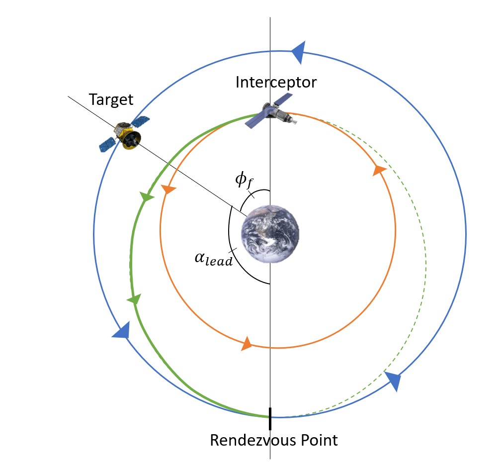
These two parameters are needed to find the lead angle, α_lead. The lead angle is the angle between the initial position of the target and the rendezvous point. The important thing to realize with this problem is that the lead angle and all the pictures shown thus far are showing this process just at the right time. It takes the same amount of time to reach the rendezvous point as the interceptor takes to complete its Hohmann Transfer.

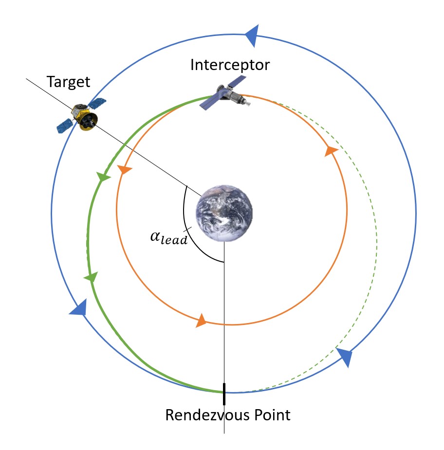
This angle can be found by taking a product of the angular velocity of the target and the time of flight of the interceptor.

[latex]\alpha_{lead} = \omega_{target}TOF[/latex]

In this particular orientation, we can also consider the final phase angle, φ_f. The phase angle is the angle between the interceptor and the target. In this final orientation, it is straightforward to find by considering the graphic below. Since the distance between the interceptor and the rendezvous point is [latex]\pi[/latex] radians (180°), and the distance between the target and the rendezvous point is defined as the lead angle, then the difference between these angles is the phase angle.

This leaves the equation to be:

[latex]\phi_{f}=\pi - \alpha_{lead}[/latex]

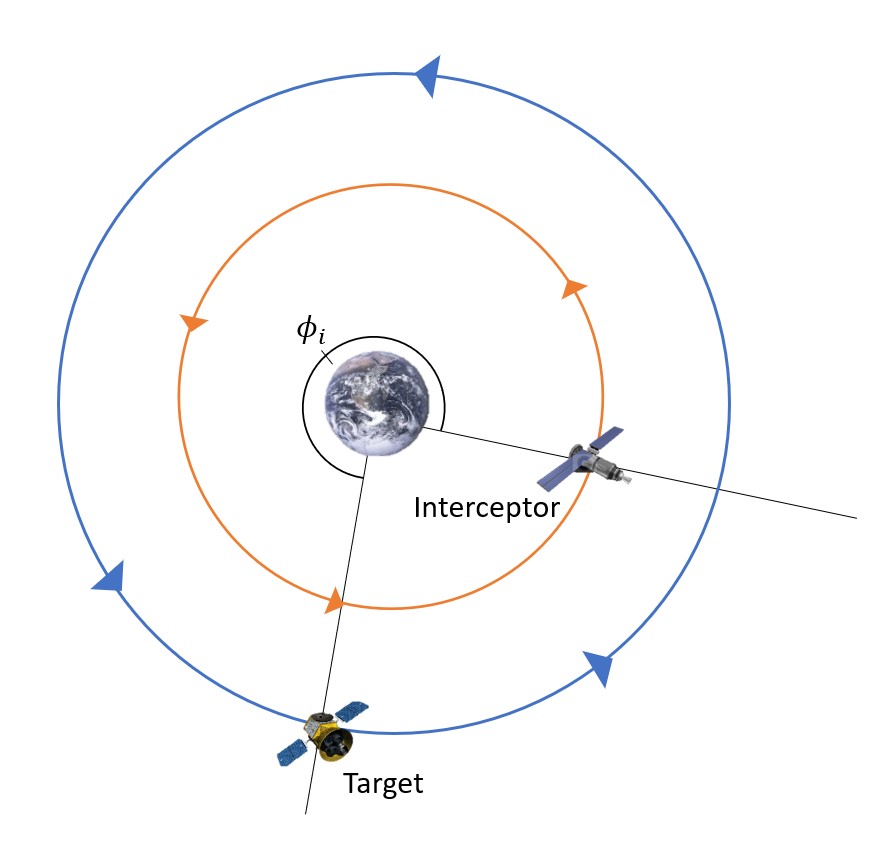
Now that the heavier back end of this problem is finished, let us consider the front end of the co-planar rendezvous problem. With the perfect time to complete this maneuver only happening at very specific times the chance that the target will be exactly where we need it in order to perform this transfer is nearly zero. As a result of this, we need to take a look at the current state of the system to determine how much time needs to pass before we are in the correct orientation. The important piece of information we need to gather from this is the initial phase angle. That is, how far is the target from the interceptor measured as an angular distance?

Between this, the final phase angle, and the angular velocities of both the interceptor and the target, a relationship can be found.

[latex]\phi_{f} = \phi_{i}\,+\,(\omega_{target} - \omega_{interceptor})\,*\,Wait\; Time[/latex]

This can be reorganized to yield:

[latex]Wait\; Time = \frac{\phi_{f} - \phi_{i}}{\omega_{target}-\omega_{interceptor}}[/latex]

Sometimes, this can yield a negative number. In that case, we simply add 2π to the numerator and recalculate, much like we did in Kepler’s Prediction Problem.

Everything shown prior to this has shown the interceptor in a smaller orbit than the target, but this can be calculated just as easy for an interceptor in a larger orbit than the target. The biggest difference is we are completing a Hohmann Transfer from a larger to smaller orbit and larger lead angles will be found.

Check your understanding with this short quiz:

EXAMPLE 1

A satellite is in distress in a circular orbit at 240 km altitude. The rescue vehicle is in a co-planar circular orbit at 120 km altitude. The rescue vehicle is 135˚ behind the target satellite.

Find the time of flight of this maneuver, the lead angle, the final phase angle, and the wait time.

CO-ORBITAL

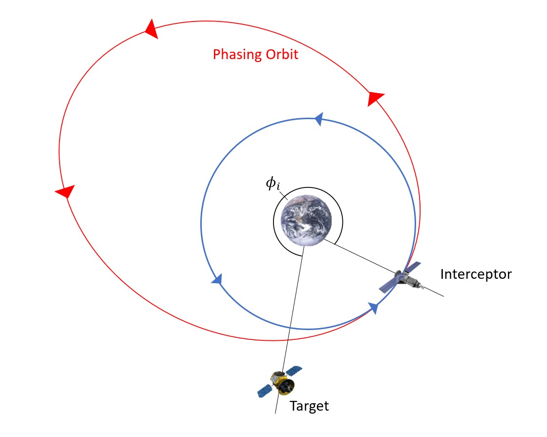
The second kind of Rendezvous maneuver occurs when the interceptor and target are in the same exact orbit, but just not in the same position. This could occur if our timing is off in the co-planar rendezvous case. In this scenario, we cannot simply perform a Hohmann Transfer at the right time to meet at a shared location. We also cannot just perform a maneuver to a straight shot to our target, as this would move the satellite into a larger orbit. What we need to do is transfer into a specific phasing orbit, which will either slow down or speed up the interceptor. Whether the interceptor satellite needs to speed up or slow down depends on whether it is ahead or behind the target in order to let the target catch up with it or to catch up with the target. This splits the problem into two different cases. Case 1 is when the target is ahead of the interceptor, and case 2 is when the interceptor is ahead of the target.

Case 1: Target Ahead of Interceptor

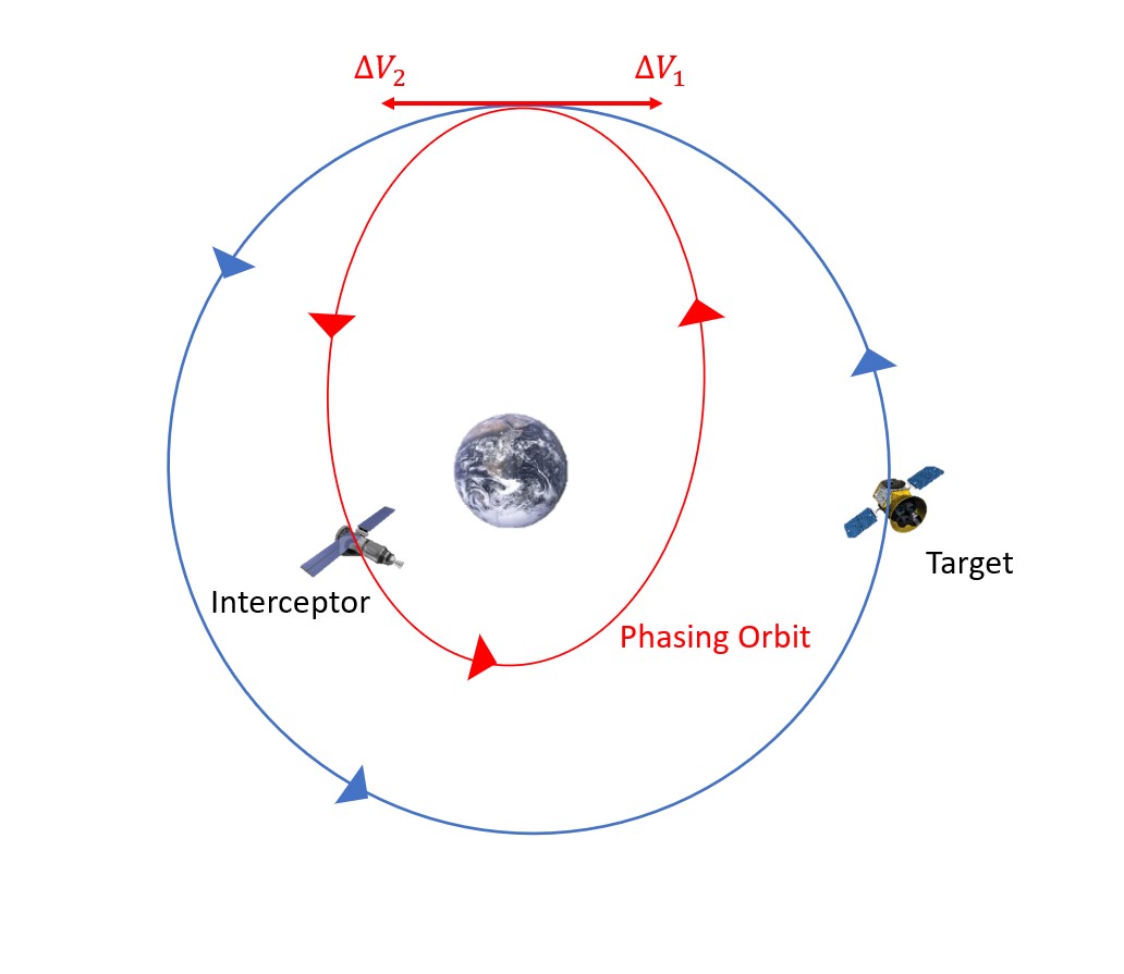
The basis of this case is that the target is ahead of the interceptor. This means that the angular distance from the interceptor to the target is less than the angular distance from the target to the interceptor (going in the same direction as the orbit). In this case, we are going to move the interceptor into a smaller phasing orbit with a smaller period. This will speed the interceptor up, and when timed correctly, it will meet back up (i.e. rendezvous) with the target after one orbit.

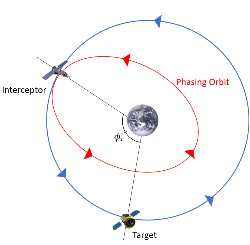
To get into this smaller phasing orbit, the interceptor must slow down. This might sound counterintuitive because we are trying to speed up. However, in order to transfer into this orbit, the satellite must slow down to speed up.

A simulation of this type of rendezvous may be seen here. The target satellite is represented by the red dot and the interceptor satellite is represented by the green dot.

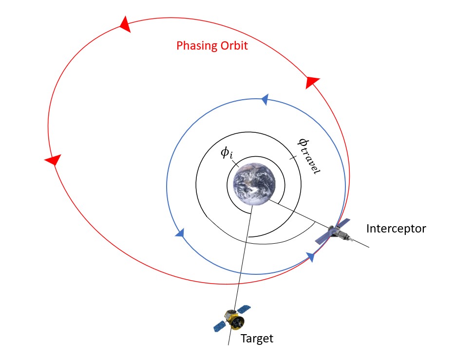
The first step in determining how to complete this maneuver is to determine how far the target will have to travel to reach the rendezvous point. We call this φ_travel. In this problem, the rendezvous point is where the interceptor starts and ends its maneuvers.

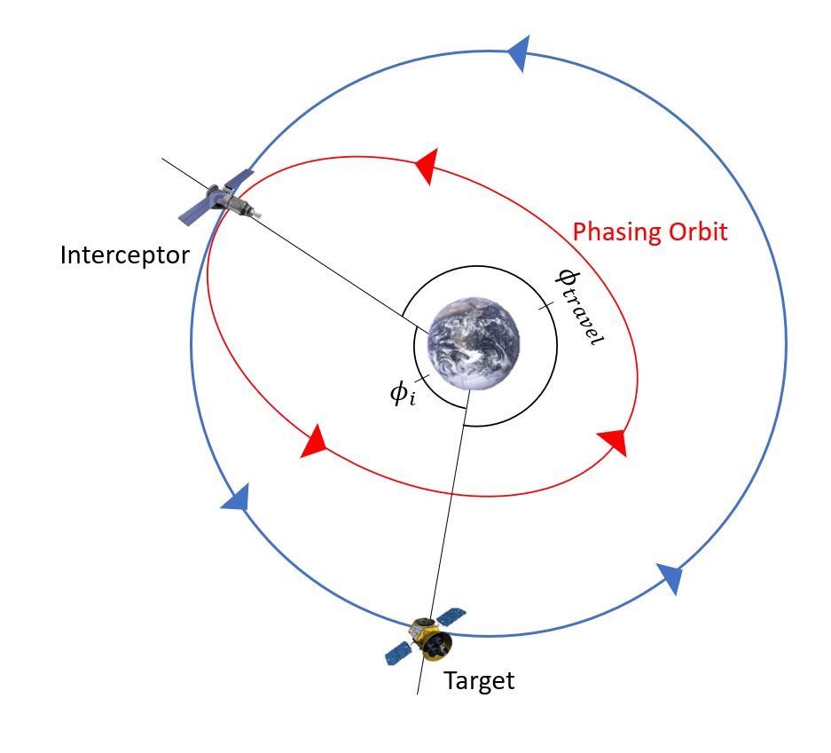
Pictorially, we can see that this angle is just the difference between one full rotation of the initial phasing angle. This is show mathematically below:

[latex]\phi_{travel}=2\pi - \phi_{initial}[/latex]

We will be using angular velocity of the target:

[latex]\omega_{target}=\sqrt{\frac{\mu}{a^3_{target}}}[/latex]

We need both of these values to calculate the time of flight of the target. This is needed because we are going to set the time for the target to travel to the rendezvous point equal to the period of the phasing orbit. In this case, the time it will take for the target satellite to travel from its current location to the rendezvous point is given by:

[latex]TOF = \frac{\phi_{travel}}{\omega_{target}}[/latex]

Next, consider the time of flight of the phasing orbit. We know it has to be the same as the time of flight, but just calculated for a successful rendezvous.

[latex]TOF = 2\pi \sqrt{\frac{a^3_{phasing}}{\mu}}[/latex]

Rearranging, we can solve for the semi-major axis of the phasing orbit:

[latex]a_{phasing}=\sqrt[3]{(\frac{TOF}{2\pi})^2\mu} = \sqrt[3]{(\frac{\phi_{travel}}{2\pi\omega_{target}})^2 \mu}[/latex]

*NOTE: This phasing orbit cannot have a radius of perigee less that ~6578 km or it will crash into the Earth. If this is the case, you will need to use case 2.

It is also important to know the change in velocities needed to successfully complete this maneuver.

First, the specific mechanical energy of the phasing orbit is needed:

[latex]\varepsilon_{phasing} = -\frac{\mu}{2a_{phasing}}[/latex]

This can then be used to find the velocity of the phasing orbit at the rendezvous point (perigee):

[latex]v_{p,phasing} = \sqrt{2(\frac{\mu}{R} \,+\, \varepsilon_{phasing})}[/latex]

Assuming circular initial and final orbits, the equation for the interceptor’s initial and final velocity is going to be:

[latex]V_{1} = \frac{\mu}{R}[/latex]

The burn for the first maneuver is:

The second burn is actually going to be the same as the first burn as the interceptor is transferring between the same two orbits. The only difference is it will be in the opposite tangential direction. This means that the total burn is:

Case 2: Interceptor Ahead of Target

This second case is the opposite of the first. The interceptor is now ahead of the target. This now means that the angular distance from the target to the interceptor is less than the angular distance from the interceptor to the target (going in the same direction as the orbit).

*NOTE: If the two distances are equal, either case may be used with the limiting factor being that the size of the smaller phasing orbit must be greater than 6578 km.

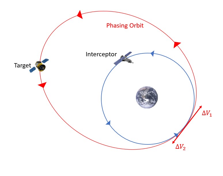
This indicates that we must now speed up to slow down. In other words, the interceptor satellite will speed up to enter into a phasing orbit larger than the initial orbit with a longer period in order to allow the target to catch up with the interceptor.

A simulation of this type of rendezvous may be seen here. Again, the target satellite is represented by the red dot and the interceptor satellite is represented by the green dot.

The largest difference this makes is that the target must travel more than a full orbit in order to catch up with where the interceptor started.

The angle that the target travels is given by:

The rest of the steps remain the same. We will still be using angular velocity of the target.

We need both of these values to calculate the time of flight of the target. The time of flights of the interceptor and the target still need to be matched.

Let us start of with the time of flight of the phasing orbit because we know it has to be the same as the time of flight just calculated.

Rearranging, we can solve for the semi-major axis of the phasing orbit:

***NOTE: The ONLY difference between this case and case 1 is the angle the target travels.

It is also important to know the burns needed to make this maneuver possible.

First, the specific mechanical energy of this orbit is needed:

This can then be used to find the velocity of the phasing orbit at the rendezvous point (perigee):

Assuming a circular initial orbit, the equation for the interceptor’s initial and final velocity is going to be:

The burn for the first maneuver is:

The second burn is also going to be the same as the first burn as the interceptor is transferring between the same two orbits. The only difference is it will be in the opposite tangential direction. This means that the total burn is:

EXAMPLE 2

A payload and its target are in the same 1,000 km altitude circular orbit and are 180° apart from each other.

Find the time of flight, the size of phasing orbit (a_phasing), and the total burn for both cases. Which case would we choose if we wanted to conserve fuel and were not as worried about time?

SOLUTIONS TO EXAMPLES:

***EXAMPLE 1 SOLUTION***

A satellite is in distress in a circular orbit at 240 km altitude. The rescue vehicle is in a co-planar circular orbit at 120 km altitude. The rescue vehicle is 135˚ behind the target satellite.

Find the time of flight of this maneuver, the lead angle, the final phase angle, and the wait time.

Solution

Solution:

To start off this problem, let us begin with understanding what has been defined by the problem. The satellite in distress is not going to be moving from its orbit. It will continue on. This tells us that this is the target. We can the find the radius of this orbit:

The rescue vehicle would then be the interceptor. Let us calculate that radius:

We are also told that the rescue vehicle is 135° behind the target satellite. This is our given initial phase angle:

To solve this problem, let us start off by determining the semi-major axis of the transfer orbit that the interceptor will travel. R_interceptor and R_target are the radii of the interceptor’s orbit and target’s orbit respectively:

This can now be used to find the time of flight:

Next, the angular velocity of both the target and interceptor should be calculated to use later. Remember that since we are assuming circular orbits, the semi-major axis and radii of these orbits are the same.

The lead angle can now be calculated:

This value can now be used to find the final phase angle:

Finally, the wait time can be calculated using all of these values.

***EXAMPLE 2 SOLUTION***

A payload and its target are in the same 1,000 km altitude circular orbit and are 180° apart from each other.

Find the time of flight, the size of phasing orbit (a_phasing), and the total burn for both cases. Which case would we choose if we wanted to conserve fuel and were not as worried about time?

Solution

Let us start off by simply finding the radius of the current orbit and the angular velocity of the target.

Let us first look at this problem from the view of case 1 where we slow down to speed up.

Case 1:

We are first going to need the big difference between the two cases and that is the angle traveled by the target. For case 1, this is:

Next, we need this time of flight:

We can now find the size of the phasing orbit:

Now to calculate the burn, staring with the specific mechanical energy of the phasing orbit:

This can then be used to find the velocity of the phasing orbit at the rendezvous point (perigee):

Assuming a circular initial orbit, the equation for the interceptor’s initial and final velocity is going to be:

The burn for the first (and second) maneuver is:

The total burn is then going to be:

A simulation of this scenario may be seen here. Note that this WILL NOT WORK because the interceptor satellite crashes into the Earth. You could also deduce that this is an unrealistic scenario as soon as you calculated a_phasing = 4647.84 km. Since it is less than the radius of the Earth, 6,738 km, it will hit the Earth.

Now for the second case where we speed up to slow down.

Case 2:

The one big change here is going to be the angle that the target travels:

Next, we need the time of flight:

We can now find the size of the phasing orbit:

Now to calculate the burn, start with the specific mechanical energy of the phasing orbit:

This can then be used to find the velocity of the phasing orbit at the rendezvous point (perigee):

Assuming a circular initial orbit, the equation for the interceptor’s initial and final velocity is going to be:

The burn for the first (and second) maneuver is:

The total burn for case 2 is then going to be:

A simulation of this scenario may be seen below.

We can see here that there is a tradeoff between burn speed (fuel) and time of flight as well as orbital size. So for this maneuver, if we wanted to conserve fuel and did not want to crash into the Earth, we would choose case 2 to speed up to slow down.

References

Bate, R. R., Mueller, D. D., & White, J. E. (2015). Fundamentals of astrodynamics. Dover Publications.

Animation of rotating Earth at night.webm. Wikimedia Commons. https://commons.wikimedia.org/wiki/File:Animation_of_Rotating_Earth_at_Night.webm

NASA. (2020, October 5). In depth. NASA. Retrieved March 28, 2023, from In Depth | Hubble Space Telescope – NASA Solar System Exploration

Sellers, J. J., Astore, W. J., Giffen, R. B., & Larson, W. J. Understanding Space An Introduction to Astronautics (3rd ed.). The McGraw-Hill Companies, Inc.

Simple graphic illustration globe showing latitude stock vector (royalty free). Shutterstock. https://www.shutterstock.com/image-vector/simple-graphic-illustration-globe-showing-latitude-13234843

Vallado, D. A., & McClain, W. D. (2013). Fundamentals of Astrodynamics and Applications. Microcosm Press.