11 Chapter 11 – Interplanetary Travel

Up to this point, we have talked about many different astrodynamics topics and maneuvers. However, none have been as challenging as traveling between planets across the solar system. This topic is what many people think about when speaking of space travel. Missions such as the Curiosity rover to Mars, New Horizons to Pluto, and Juno, which traveled to Jupiter, are examples of this topic.

All of these missions began here on Earth and traveled millions and even billions of kilometers to reach their destinations. The image below shows an overview of these types of missions. Notice an alarming aspect of this image is that there are four bodies, but we have only worked with two body problems up to this point!

The scale of these missions might seem daunting, but it is possible to solve these problems based on the information we already know. Instead of focusing on the mission as a whole, we will use the method of breaking the trajectory up into three different sections called the pathed-conic approximation. To begin, we will make the assumption that the orbits of every planet around the Sun are circular. However, as discussed previously, no orbit is perfectly circular. The highest eccentricity belongs to Mercury of ~0.2, and all other planets’ orbits have an eccentricity of less than 0.1. Nonetheless, it is not a bad assumption to make.

REGION 1: SUN-CENTERED TRANSFER 

After we have left the earth’s sphere of influence and before arriving at the target planet’s sphere of influence, the first region we are going to look at is the Sun-centered transfer. This means that we are going to use the Sun as the central body (which we call heliocentric) just as we have treated the earth as our central body in previous chapters. Therefore, we need to establish a new gravitational constant. Previously, we have used the generic μ as the gravitational constant equal to 398,600.5 km³/s². However, now we have to make the distinction of what the central body is. In this first region, with the Sun as the central body, the new gravitational constant is defined as:

μ_Sun = 1.3271544×10¹¹ km³/s²

Another important variable to define is the radius from the center of the Sun to the center of the earth. The distance from the center of the earth to the center of the target planet is also important, but that value is going to change for every planet. The average distance from the Sun to the earth is:

R_toEarth = 1.496×10⁸ km

With these two variables defined, let us consider the entire Region 1 figure below:

As it can be seen in the image above, this part of the process is simply a two-body system with the two bodies being the Sun and the spacecraft. It might also be noticed that this looks a lot like a Hohmann transfer between two circular orbits. This transfer orbit is heliocentric (which means we are looking at all the velocities with respect to the Sun).

The first step in the algorithm for Region 1 is determining how fast the earth is traveling. Note at this point we are going to assume the spacecraft is in some initial parking orbit around Earth. Because we are now looking at velocities with respect to the Sun, the spacecraft’s initial orbit around the earth is going to appear to have nearly the same velocity as the earth is moving around the Sun. Therefore, what we defined as V₁ in the Hohmann transfer section of chapter 7 is now going to be called V_Earth and we are going to define it using the equation of velocity of an object in a circular orbit.

[latex](1) V_{Earth} = \sqrt{\frac{\mu_{Sun}}{R_{toEarth}}}[/latex]

The next step is to determine the size and specific mechanical energy of the transfer orbit. This is no different than the previous case of the Hohmann transfer. However, in this case, perigee is at the earth and apogee is at the target planet.

[latex]a_{t} = \frac{R_{toEarth} + R_{toTarget}}{2}[/latex]

[latex](2)[/latex] [latex]\varepsilon_{t} = - \frac{\mu_{Sun}}{2a_{t}}[/latex]

As soon as we enter this heliocentric transfer orbit when we have left the earth’s sphere of influence, we are traveling at a new velocity, which we will call V_trans@Earth. This is very similar to the V_t1 seen in chapter 7. We use the distance from the Sun to the earth and the specific mechanical energy we just calculated of the transfer orbit to determine what the velocity needs to be at this point in the transfer orbit.

[latex](3)[/latex] [latex]V_{trans@Earth} = \sqrt{2(\frac{\mu_{Sun}}{R_{toEarth}} + \varepsilon_{t})}[/latex]

Notice in the figure that defines this region that we need to add velocity to the initial velocity of the earth to get to the velocity of the transfer orbit. In a generic Hohmann transfer problem, we would call this velocity change the Delta V burn, but we are going to give this one a slightly different name of V_∞Earth. It will become apparent soon why we do this.

[latex](4)[/latex] [latex]V_{\infty Earth} = \left| V_{trans@Earth} - V_{Earth} \right|[/latex]

Now, let us focus on the other side of this transfer orbit– arrival at the target planet. We will start by calculating the planet’s velocity around the Sun just as we did the earth. Note that μ_Sun will be the same, but R_toTarget will not be.

[latex](5)[/latex] [latex]V_{target} = \sqrt{\frac{\mu_{Sun}}{R_{toTarget}}}[/latex]

Similar to before, we want to find at what velocity the spacecraft will be traveling at the end of its transfer orbit. The specific mechanical energy will be the same at this location as it is constant for any orbit.

[latex](6)[/latex] [latex]V_{trans@target} = \sqrt{2(\frac{\mu_{Sun}}{R_{toTarget}} + \varepsilon_{t})}[/latex]

We are also going to find the difference between these velocities of V_∞Target. It should be noted that this is defined slightly different than V_∞Earth. It just has V_∞Planet and V_planet flipped.

[latex](7)[/latex] [latex]V_{\infty Target} = \left| V_{target} - V_{trans@target} \right|[/latex]

The last piece of information that would be needed for this region of the mission is the time of flight. Some very large numbers might occur with this calculation. However, remember that we are traveling very large distances, so very large time of flights in seconds will be normal.

[latex](8)[/latex] [latex]TOF = \pi \sqrt{\frac{a^{3}_{t}}{\mu_{sun}}}[/latex]

REGION 2: EARTH DEPARTURE 

The second region we want to focus on is where we are departing the earth’s sphere of influence. Isolating the problem down to the image seen below, we can see that this section also has only two bodies — one being the earth and the other the spacecraft. This also puts the coordinate system back into the geocentric equatorial one we are used to seeing.

This problem might seem unfamiliar, but we have actually looked at this once before in chapter 2. It might have been difficult at the time, but with our new set of knowledge, this process should go smoothly. We are going to define the orbit of the spacecraft’s exit trajectory to be a hyperbolic one. It is going to start in some parking orbit, V_park@Earth , and enter the hyperbolic orbit in order to reach an exit velocity of V_∞Earth , which should look familiar.

The first piece of information that can be easily calculated is the velocity of the spacecraft in Earth’s parking orbit, which we are going to assume is circular.

[latex]V_{park@Earth} = \sqrt{\frac{\mu_{Earth}}{R_{park@Earth}}}[/latex]

We now want to enter this hyperbolic orbit, but it may seem like we have very little information on it. However, we have all the information we need. In this hyperbolic obit, the satellite needs to be traveling at an escape velocity of V_∞Earth at the edge of the earth’s sphere of influence. We define the sphere of influence to have such a large radius, (we can estimate as approximately 1 million km) so we can justify calling it infinity. Now, let us try to calculate specific mechanical energy with this information. We can see that a fraction with infinity in the denominator just goes to 0. 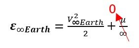This leaves us with a specific mechanical energy of the hyperbolic orbit to be just a function of V_∞Earth , which we calculated in Region 1! Notice this energy will always be positive.

[latex]\varepsilon_{\infty Earth} = \frac{V^{2}_{\infty Earth}}{2}[/latex]

As always, specific mechanical energy is the same anywhere on an orbit, so we can use this to find what the velocity needs to be at the park orbit to enter the hyperbolic orbit. This point will still have the same radius as the parking orbit. We are going to use the notation of V_hyp@Earth. Make sure not to confuse this with V_∞Earth as it is still the velocity in the hyperbolic orbit. It is just at a very different location.

[latex]V_{hyp@Earth} = \sqrt{2(\frac{\mu_{Earth}}{R_{park@Earth}} + \varepsilon_{\infty Earth})}[/latex]

We can then calculate the actual burn it will take to “boost” the spacecraft from the park orbit to the hyperbolic orbit by taking the difference of these two velocities.

[latex]\bigtriangleup V_{boost} = \left| V_{hyp@Earth} - V_{park@Earth} \right|[/latex]

Region 3: Target Arrival

Now, let us look at the other end of this mission — the arrival at the target planet. Looking at the figure below, it looks incredibly similar to the departure of Earth, just backwards. This region is also a two-body system with the spacecraft and the target planet being the two bodies. This time, the coordinate system is target centered. MAKE SURE TO USE THE CORRRECT GRAVITATIONAL CONSTANT, μ, FOR THIS PLANET!

Again, this is just the reverse of what we did in the earth departure region. We will be moving from a hyperbolic orbit from the sphere of influence to the target’s park orbit, which we will again define as circular. We can easily calculate the final velocity of the park orbit given its distance from the center of the planet:

[latex]V_{park@Target} = \sqrt{\frac{\mu Target}{R_{park@Target}}}[/latex]

We also want to find the specific mechanical energy of the hyperbolic orbit, again assuming that the radius is infinite, which would leave the equation in terms of V_∞Target.

[latex]\varepsilon_{\infty Target} = \frac{V^{2}_{\infty Target}}{2}[/latex]

As always, specific mechanical energy is constant and can be used to calculate what the velocity of the spacecraft at the parking orbit in the hyperbolic orbit.

[latex]V_{hyp@Target} = \sqrt{2(\frac{\mu_{Target}}{R_{park@Target}} + \varepsilon_{\infty Target})}[/latex]

We can now use the difference between the two velocities at this point to calculate the retro burn needed to change from the hyperbolic orbit to the final parking orbit.

[latex]\Delta V_{retro} = \left| V_{hyp@Target} - V_{park@Target} \right|[/latex]

Big Picture

One parameter that would be important to this type of mission is to find the total burn of the entire mission. We truly only had two burns: the boost burn and the retro burn. If we take the sum of these values, we will get the burn of the entire mission.

[latex]\Delta V_{Mission} = \Delta V_{Boost} + \Delta V_{Retro}[/latex]

EXAMPLE 1

Take the example of traveling from the Earth to Saturn. It starts at a paring orbit on Earth at a radius of 6,678 km and ends at a parking orbit around Saturn at a radius of 63,268 km. Find the total burn needed for the mission. The distance from the center of the Sun to the center of Saturn is 1,427×10⁶ km and Saturn’s gravitational constant is μ_Saturn = 3.7967×10⁷ km³/s².

Now that we are no longer just looking at the earth, we need a way to distinguish between the different planets without writing the whole name out. So instead of names, we use symbols. Ironically, the earth’s is a target, which does not look good for us if any aliens are planning on doing any interplanetary travel. The symbols of the eight planets can be seen in the following image:

Try out this quiz:

SOLUTIONS TO EXAMPLES:

***EXAMPLE 1 SOLUTION***

Take the example of traveling from the earth to Saturn. It starts at a paring orbit on Earth at a radius of 6,678 km and ends at a parking orbit around Saturn at a radius of 63,268 km. Find the total burn needed for the mission. The distance from the center of the sun to the center of Saturn is 1,427×10⁶ km and Saturn’s gravitational constant is μ_Saturn = 3.7967×10⁷ km³/s².

Solution

Remember that:

[latex]\mu_{Sun} = 1.3271544 \times 10^{11} \frac{km^{3}}{s^{2}}[/latex]

[latex]R_{toEarth} = 1.496 \times 10^{2} km[/latex]

We need these values to start Region 1: The Sun centered transfer in order to determine V_∞ for both the earth and Saturn. We just need to follow the algorithm.

(1) [latex]V_{Earth} = \sqrt{\frac{\mu_{Sun}}{R_{toEarth}}} = \sqrt{\frac{1.3271544 \times 10^{11} \frac{km^{3}}{s_{2}}}{1.496 \times 10^{8}km}} = 29.78 km/s[/latex]

[latex]a_{t} = \frac{R_{toEarth} + R_{toTarget}}{2} = \frac{1.496 \times 10^{8}km + 1427 \times 10^{6}km}{2} = 7.883 \times 10^{8} km[/latex]

(2) [latex]\varepsilon_{t} = -\frac{\mu_{Sun}}{2a_{t}} = \frac{1.327 \times 10^{11} \frac{km^{3}}{s^{2}}}{2(7.883 \times 10^{8} km)} = -81.16846378\frac{km^{2}}{s^{2}}[/latex]

(3) [latex]V_{trans@Earth} = \sqrt{2(\frac{\mu_{Sun}}{R_{toEarth}} + \varepsilon_{t})} = \sqrt{2(\frac{1.327 \times 10\frac{km^{3}}{s^{2}}}{1.496 \times 10^{8}km} - 84.16846478\frac{km^{2}}{s^{2}})} = 40.0715 km/s[/latex]

(4) [latex]V_{\infty Earth} = \left| V_{trans@Earth} - V_{Earth} \right| = \left| 40.07152659 km/s - 29.781 km/s \right| = 10.29 km/s[/latex]

(5) [latex]V_{target} = \sqrt{\frac{\mu_{Sun}}{R_{toTarget}}} = \sqrt{\frac{1.327 \times 10^{11} \frac{km^{3}}{s^{2}}}{1427 \times 10^{6} km}} = 9.64325 km/s[/latex]

(6) [latex]V_{trans@target} = \sqrt{2(\frac{\mu_{Sun}}{R_{toTarget}} + \varepsilon_{t})} = \sqrt{2 (\frac{1.327 \times 10^{11}\frac{km^{3}}{s^{2}}}{1427 \times 10^{6}km} - 84.16846378\frac{km^{2}}{s^{2}})} = 4.2 km/s[/latex]

(7) [latex]V_{\infty Target} = \left| V_{target} - V_{trans@target} \right| = \left| 9.64325 km/s - 4.2 km/s \right| = 5.44234 km/s[/latex]

(8) [latex]TOF = \pi \sqrt{\frac{a^{3}_{t}}{\mu_{sun}}} = \pi\sqrt{\frac{(7.883 \times 10^{8}km)^{3}}{1.327 \times 10^{11}\frac{km^{3}}{s^{2}}}} = 190876165.2s = 6.0526 years[/latex]

Now let us take a look at Region 2: Earth departure.

[latex]V_{park@Earth} = \sqrt{\frac{\mu_{Earth}}{R_{park@Earth}}} = \sqrt{\frac{398600.5\frac{km^{3}}{s^{2}}}{6678 km}} = 7.72584 km/s[/latex]

[latex]\varepsilon_{\infty Earth} = \frac{V^{2}_{\infty Earth}}{2} = \frac{(10.29km/s)^{2}}{2} = 52.94205 km/s[/latex]

[latex]V_{hyp@Earth} = \sqrt{2(\frac{\mu_{Earth}}{R_{park@Earth}} + \varepsilon_{\infty Earth})} = \sqrt{2(\frac{398600.5\frac{km^{3}}{s^{2}}}{6678 km} + 52.94205\frac{km^{2}}{s^{2}})} = 15 km/s[/latex]

[latex]\bigtriangleup V_{boost} = \left| V_{hyp@Earth} - V_{park@Earth} \right| = \left| 15 km/s - 7.72584 km/s \right| = 7.28287 km/s[/latex]

Finally, we can look at the final region: Saturn arrival.

[latex]V_{park@Target} = \sqrt{\frac{\mu_{Target}}{R_{park@Target}}} = \sqrt{\frac{3.7967 \times 10^{7}\frac{km^{3}}{s^{2}}}{63268 km}} = 24.497 km/s[/latex]

[latex]\varepsilon_{\infty Target} = \frac{V^{2}_{\infty Target}}{2} = \frac{(5.44234 km/s)^{2}}{2} = 14.8095\frac{km^{2}}{s^{2}}[/latex]

[latex]V_{hyp@TArget} = \sqrt{2(\frac{\mu_{Target}}{R_{park@Target}} + \varepsilon_{\infty Target})} = \sqrt{2(\frac{3.7967 \times 10^{7}\frac{km^{3}}{s^{2}}}{63268 km} + 14.8095\frac{km^{2}}{s^{2}})} = 35.0687 km/s[/latex]

[latex]\bigtriangleup V_{retro} = \left| V_{hyp@Target} - V_{park@TArget} \right| = \left| 35.0687 km/s - 24.497 km/s \right| = 10.5717 km/s[/latex]

Putting these two burns together, we can find the total burn of the whole mission.

[latex]\bigtriangleup V_{Mission} = \bigtriangleup V_{Boost} + \bigtriangleup V_{retro} = 7.28287 km/s + 10.5717 km/s[/latex]

[latex]\bigtriangleup V_{Mission} = 17.8546 km/s[/latex]

REFERENCES

Bate, R. R., Mueller, D. D., & White, J. E. (2015). Fundamentals of astrodynamics. Dover Publications.

Animation of rotating Earth at night.webm. Wikimedia Commons. https://commons.wikimedia.org/wiki/File:Animation_of_Rotating_Earth_at_Night.webm

“Perifocal Frame.” Perifocal Frame – Orbital Mechanics & Astrodynamics, https://orbital-mechanics.space/classical-orbital-elements/perifocal-frame.html.

Sellers, J. J., Astore, W. J., Giffen, R. B., & Larson, W. J. Understanding Space An Introduction to Astronautics (3rd ed.). The McGraw-Hill Companies, Inc.

Simple graphic illustration globe showing latitude stock vector (royalty free). Shutterstock. https://www.shutterstock.com/image-vector/simple-graphic-illustration-globe-showing-latitude-13234843

Vallado, D. A., & McClain, W. D. (2013). Fundamentals of Astrodynamics and Applications. Microcosm Press.