1 Chapter 1 – Orbital Basics

Welcome to chapter 1! In this chapter we will investigate the basis for satellite motion. We will start with a brief history of some individuals who helped us initially understand the reason objects in space, including planets, move the way they do. We will then look at the laws of two famous individuals who were great contributors to the world of astrodynamics, namely Isaac Newton and Johannes Kepler. We will then combine two of these laws – including Newton’s Second Law and his Universal Law of Gravitation, to develop the two-body equation of motion, which will form the basis for our study of orbital mechanics.

Objectives for this chapter are:

• Explain how early space explorers contributed to our understanding of orbits.
• Understand Newton’s three basic laws of motion and how they apply to orbits.
• Explain and use Newton’s Universal Law of Gravitation.
• Use the two constants of orbital motion – specific mechanical energy and specific angular momentum, to explain basic properties of orbits.
• Combine these laws to develop the two-body equation of motion.
• Integrate the two-body equation of motion (optional).

Before you proceed, you may want to review some of the basics of vector mathematics, trigonometry and calculus. Here is some background information you may find useful:

EARLY ASTRONOMERS AND KEPLER’S LAWS

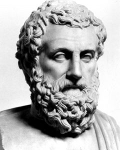
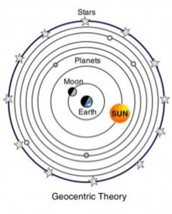
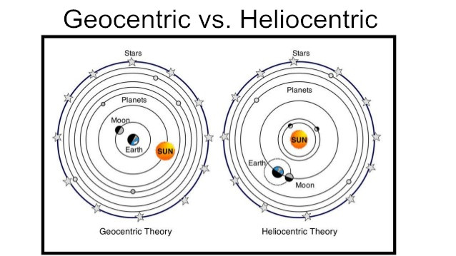
Some of the earliest contributors to understanding space were early philosophers, such as the Greek philosopher Aristotle, who lived from 384 – 322 BC. For nearly 2,000 years, his view of a stationary Earth at the center of a revolving universe, in other words a geostatic and geocentric universe, dominated the world’s thinking on the subject. This view of the universe became engrained in Christian theology, making it a doctrine of religion (Team, 2018).

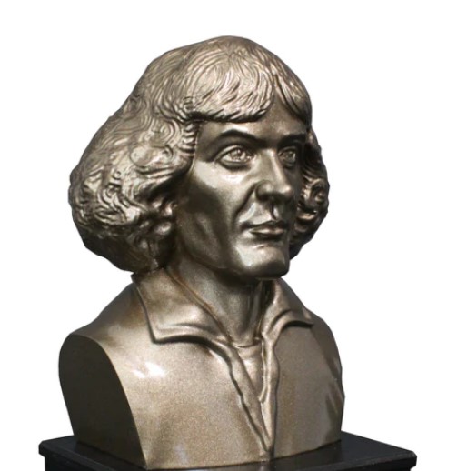
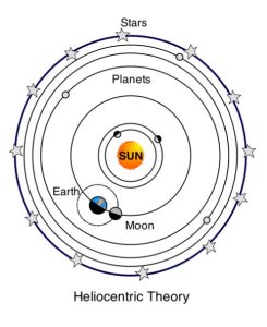
Nicolaus Copernicus, a Polish astronomer, was born in 1473. As a teenager, supposedly his parents, like thousands of parents since then, finally got tired of his self-centeredness and said “Son, the universe doesn’t revolve around you!” That gave him a deep philosophical dilemma to ponder. It is believed that Copernicus probably hit upon his main idea sometime in the early 1500s and wrote a manuscript called Commentariolus, or in English, “Little Commentary.” In this work, he proposed the Sun as the fixed point around which the planets rotate in circular orbits. He also proposed that the earth turns once daily on its own axis. His system was quickly denounced by both Catholics and Protestants. However, his heliocentric, or Sun-centered view of the universe had tremendous consequences for later thinkers of the Scientific Revolution, including major figures like Galileo, Kepler, and Newton.

Tycho Brahe, who lived from 1546 – 1601, was more of a traditional observational astronomist. Brahe was quite an eccentric individual who took his work quite seriously. Although he still believed the planets orbited in circular orbits around the sun, he also believed the sun, moon, and stars circled the earth. He was known for taking very meticulous measurements of the objects in the heavens. His scientific accomplishments include the discovery of the supernova in 1572 and a series of essays on the movement of comets.

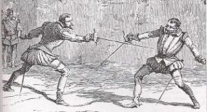
A wealthy man of noble birth, Brahe owned a significant amount of all the money in Denmark and used it to fund his projects. He was also known for being hot-headed and was in a heated discussion about mathematics over ales when he was challenged to a duel. Not one known to duck out of a challenge, he agreed to the duel while intoxicated and lost his nose in 1566. Brahe simply purchased an expensive replacement made of a brass, or possibly even a gold-silver alloy, which is why he has a strange looking nose in his later photos.

Brahe also used his money to obtain the best observing instruments of his time. He met a promising young man named Johannes Kepler, and in 1600, he hired him as an assistant.  Together, they began working on a new star catalog. This catalog was eventually published by Kepler in 1627 as the Rudolphine Tables. They were by far the most accurate astronomical data ever published, which included not only planetary data, but also the positions of 1,006 stars. The majority of these stars were cataloged to within one arc minute of accuracy. To understand this, take a circle and divide it into 360 equal parts to get one minute of accuracy. Then divide each minute in 60 parts! In other words, this is 1/60th of one degree.

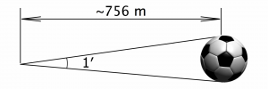
To give you an idea of the accuracy of these measurements, a standard soccer ball with a diameter of 22 cm or 8.7 in subtends and angle of 1 arcminute at a distance of approximately 756 meters, or 827 yards!

Brahe was responsible for multitudes of precise measurements, but was not a skilled mathematician. Fortunately, Kepler was; however, the Brahe-Kepler collaboration would be short-lived. In October 1601, Brahe was invited to a royal banquet. As was customary, guests were not allowed to leave the banquet table until after the king left. After Brahe consumed a huge meal and did a lot of drinking, it is believed his bladder may have burst. He suffered several days and then died. However, before his death, he challenged Kepler to calculate the orbit of Mars. It was a well-chosen task, because Mars’ orbit happens to be one of the most eccentric, or non-circular, in our solar system. (Randolph, 2017).

JOHANNES KEPLER

Kepler found a slight problem with the measurements of Mars’ orbit. The meticulous measurements Brahe had taken indicated that Mars’ orbit was not circular. It was off by eight minutes of arc between an ideal circular orbit and Brahe’s observations. Kepler began to think about the discrepancy and finally came to the conclusion that the planets moved around the Sun in elliptical orbits with the Sun not at the center, but at one of the ellipse’s focal points. Kepler was so convinced he was correct that he developed three Laws of Orbital Motion.

KEPLER’S FIRST LAW

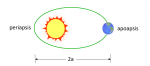
The orbits of the planets are ellipses with the Sun at one focus.

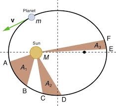
Furthermore, by studying more closely the individual parts of Mars orbits, there were differences in the time it took for the planet to travel the same distance throughout its orbit. Kepler noticed that a line between the planet and Mars swept out an equal area in an equal amount of time.   To account for this, he reasoned that when the planet is closest to the Sun, or at perihelion, it must be travelling  faster than when it is farther from the Sun.  This became Kepler’s Second Law.

KEPLER’S SECOND LAW

Planets sweep out equal areas in equal times.

Kepler published these first two laws in 1609, then ten years later he discovered his third law.

KEPLER’S THIRD LAW

The square of the orbital period, or the time it takes for a planet to complete one orbit, is directly proportional to the cube of the mean or average distance between the Sun and the  planet.

Kepler’s Third Law allows us to predict the orbit of any object in space traveling around a central body. We will later find that this relationship can be quantified by the period equation:

[latex]Period = 2\pi \sqrt{\frac{a^{3}}{\mu }} seconds[/latex]

Where

[latex]a[/latex] is the semi-major axis, which describes the size of the orbit

and

[latex]\mu = GM[/latex] is called the gravitational constant [latex]G[/latex] is the universal gravitational constant and [latex]M[/latex]is the mass of the central body.  This unsurprisingly means that the larger the orbit,  the longer it takes for the object to traverse it   For Earth, this gravitational constant is approximately 398,600.5 km³/s².  We will learn more about these parameters when we study Newton’s Universal Law of Gravitational later in this chapter.

Early Astronomers and Kepler’s Laws Video

ISAAC NEWTON

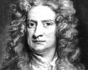
Kepler explained how the planets moved, but it was not until Isaac Newton, who lived from 1642 – 1727, that we came to understand why. In 1665, a great plague ravaged England and shut down universities. In that single year alone, Newton made significant advances in calculus, gravitation, and optics at the age of twenty-three!

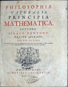
Newton finally published his three laws of motion and the Universal Law of Gravitation in Principia in 1687.

NEWTON’S FIRST LAW OF MOTION

A body continues in its state of rest, or of uniform motion in a straight line, unless compelled to change that state by forces impressed upon it.

This law says that any object which is at rest will stay at rest unless some force makes it move. Similarly, any object in motion will stay in motion forever, with a constant speed in a straight-line direction, until some force makes it change its speed or direction of motion.

This allows us to draw two conclusions on how this law applies to satellites in orbit. First, notice that a satellite is traveling in a circle or ellipse about some central body. Since it is not traveling in a straight line, there must be some force acting on it. That force is gravity, and it must be pulling the satellite in the direction of the central body. Second, inertia keeps an object from moving without the application of an outside force. However, once it is moving, an object has momentum, which is the amount of resistance an object in motion has to changes in its speed or direction of motion. We will study this more shortly, but these two conclusions can be summarized as:

1. There must be a force on satellites – gravity!
2. Momentum is conserved – orbits are constant in orientation.

At this time, it is worthwhile to review the concept of momentum.

Momentum is the amount of resistance an object in motion has to changes in its speed or direction of motion. There are two types: Linear momentum and angular momentum. We will discuss angular momentum later in this chapter.

Linear momentum is defined as mass times velocity and often represented by the variable .  In equation form, this becomes:

[latex]\vec{p} = m\vec{V}[/latex]

Where:

[latex]\vec{p} = \text{linear momentum vector} \left( \frac{\text{kg} \cdot \text{m}}{\text{s}^2} \right)[/latex]

[latex]m = \text{mass (kg)}[/latex]

[latex]\vec{V} = \text{velocity vector} \left( \frac{\text{m}}{\text{s}} \right)[/latex]

Understanding this concept leads us into Newton’s next law.

NEWTON’S SECOND LAW OF MOTION

The time rate of change of an object’s momentum is equal to the applied forces.

But is this law not simply F = ma? No!

Look closely at what Newton’s second law really says. The time rate of change of an object’s momentum is equal to the applied forces. There are two important differences here. First, we just learned that linear momentum is a vector.

[latex]\vec{p} = m\vec{V}[/latex]

The time rate of change of the momentum is then the derivative of the product of mass and velocity, or:

We can then expand this equation using the product rule from calculus:

And Newton’s second law says this product is equal the applied forces, which can be one or more, so we will use the summation symbol ∑ to write this as:

The second term,

where    is the acceleration vector.  But what about the first term? Notice that  = 0 only if mass is not changing. Then, Newton’s 2nd law takes the more familiar form:

Only when mass is not changing!

1. This has relevance to space systems in two ways:
   1. We will combine this with Newton’s Universal Law of Gravitation to form the two-body equation of motion.
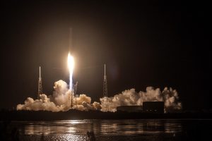
   2. In rockets, , is a large part of the thrust effect!

NEWTON’S THIRD LAW OF MOTION

For every action there is an equal and opposite reaction.

This principle of action and reaction applies universally for all mechanical systems. This is relevant to space systems in two main ways:

1. In a free-fall environment, an astronaut must be very conscious of this fact. For example, if an astronaut turns a screwdriver one way, he or she will turn the opposite direction unless anchored.
2. This is what makes rockets work – the rate at which the mass of working fluid is expelled from the engine in one direction creates thrust to the engine in the opposite direction.

NEWTON’S UNIVERSAL LAW OF GRAVITATION

Newton was not responsible for discovering gravity. After all, it was known at this time that the force of gravity caused earthbound objects (such as falling apples) to accelerate towards the earth at a rate of 9.8 m/s².  t was also known that the Moon accelerated toward the earth at a rate of 0.00272 m/s².  Newton wondered what it was about the force of gravity that caused the much more distant moon to accelerate at a rate that is approximately 1/3600 of the acceleration of an apple? In equation form:

Newton knew that the force of gravity must somehow be related to the distance between the two bodies.

The dilemma is solved by comparing the distance from the apple to the center of the earth with the distance from the Moon to the center of the earth. As the Moon revolves around the earth, it is approximately 60 times further from the earth’s center than the apple is. So, the force of gravity between the earth and any object is inversely proportional to the square of the distance that separates the object from the earth’s center. The Moon, being 60 times further away than the apple, experiences a force of gravity that is  times that of the apple.

But Newton’s Universal Law of Gravitation does not just apply to objects near the earth. As the name implies, it is universal. All objects attract each other with a force of gravitational attraction, and that force is directly dependent upon the masses of both objects and inversely proportional to the square of the distance that separates their centers. In equation form, this becomes:

Notice, R, is the distance between the two object’s centers. It turns out that there is a proportionality constant that applies throughout the universe.

Where G represents the universal gravitational constant .  The value of G was determined experimentally by Henry Cavendish in the century after Newton’s death.

Since we will be applying this equation a lot to our studies about satellites around the earth, we will define a new parameter, called the Earth’s gravitational constant,

So, Newton’s Universal Law of Gravitation for an object around the earth becomes:

Next, we will consider the laws of conservation of energy and conservation of angular momentum.

Newton’s Laws Videos

LAWS OF CONSERVATION

There are certain things that are constant in life besides the facts that we must pay taxes and that time moves forward.  Many of the basic properties we have discussed, such as momentum and energy, remain constant. In physics, if a certain property or quantity remains unchanged for a system, that property or quantity is said to be conserved.

SPECIFIC ANGULAR MOMENTUM

We learned earlier that linear momentum is conserved for a system.

Momentum is the amount of resistance an object in motion has to a change in its speed or direction of motion. But what about objects that are spinning? They also have a property  called angular momentum that is conserved. First, let us see where angular momentum comes from.

The moment of momentum, or angular momentum, is given by:

Which is always perpendicular to the plane of motion.

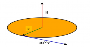
For a satellite in orbit around the earth, the orbit is in a plane, so the cross product is always perpendicular to the plane.

Now, since mass does not matter in free fall, let use define a more useful variable.

Where is specific angular momentum.

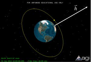
This property has huge implications for satellites in orbit.

1. A satellite’s orbital plane is fixed unless an external torque is applied.
2. It takes a LOT of energy to change an orbital plane.

Just like when you first rode a bike, you found that the faster you went, the easier it was to remain upright. This gyroscopic stability keeps an object spinning in circular motion in the same plane. As an example, consider a bicycle wheel moving forward at 20 km/hr., or 5.6 m/s. If we assume an average bicycle wheel has a mass of 2 kg and a diameter of 0.6 meters, its angular momentum is about 7 kg m²/s.

Now think about how fast spacecraft circles the earth. In a low Earth orbit at an altitude of 300 km, this is incredibly fast at approximately 7.7 km/s, or over 17,000 mph! In this this case the specific angular momentum, not including mass, is about 51,500 km²/s! It is difficult to get a feel for this, but for a typical satellite at this speed, it would take as much propellant as the spacecraft’s mass to change its orbital tilt by a mere 15^◦. For even a small satellite with a mass of 500 kg, this would be 500 kg of propellant! So how do we make these orbital tilt changes? We will discuss that later in this book.

SPECIFIC MECHANICAL ENERGY

We know a lot now about energy. It can take many forms including nuclear energy, thermal energy, electrical energy, magnetic energy, and chemical energy. Orbital mechanics is mostly governed by mechanical energy, so we will concentrate on that for now.

We know total mechanical energy consists of kinetic and potential energy.  As an example, when an object is tossed in the air, upon release energy is conserved, i.e. the system is trading kinetic and potential energy, while the total energy remains constant. The system has its smallest potential energy and greatest kinetic energy upon release upwards, but it slows down, and in fact comes to a complete stop at the very top of the toss. There, kinetic energy, at least instantaneously, is zero. Where did the energy go? It is transitioned into potential energy since it is further from the ground.

So, total mechanical energy is equal to the combination of kinetic and potential energy, and those two energies are traded off such that the total energy is constant.

E = KE + PE

Where:

E = total mechanical energy

KE = kinetic energy

PE = potential energy

From physics, we know:

KE = ½ mV² (kg m²/s²)

PE = mgh (kg m²/s²)

Where:

m = mass

V = velocity

g = gravitational constant = 9.81 m/s² (for earth)

h = height from datum (datum is where you define PE = 0)

We will define specific mechanical energy, typically in units of km²/s², as:

Recall KE = ½ mV² so the specific kinetic energy term becomes V²/2.

Also recall PE = mgh where g is the gravitational acceleration, or the acceleration at which objects near the earth fall. Using the expression for the force of gravity from earlier and setting it equal to the mass of the object times its acceleration, in this case, g, we get:

So, we see the magnitude of the gravitational constant may be written as:

Since this is acting toward the center of the earth and we measure R from there, this acts in the negative direction, or:

So,

And dividing by mass and simplifying yields the specific potential energy term:

So specific mechanical energy becomes:

Since remains constant, this is related to the constant orbital size, a, or semi-major axis by:

For a detailed derivation of this relationship, see Sellers Appendix C.4.

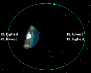
There are three important conclusions we can draw from this:

1. Since specific mechanical energy is constant, the size of the orbit, a, is constant:
2. KE and PE are traded off as the satellite travels around the orbit, so the satellite is moving fastest at its closest point to the earth, i.e. at perigee, and slowest at its farthest point from Earth, i.e. at apogee.
3. Potential energy is defined as negative until the object travels very, very far away from the earth.

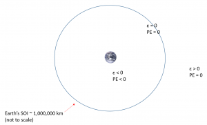
Let us consider this last point more closely. First, we see that the potential energy term becomes zero only as R approaches infinity. This would theoretically mean that the object still has potential energy until it is infinitely far away from the earth. We will establish a more practical definition for “infinitely far” as the earth’s sphere of influence, which for our purposes we will define at approximately 1 million km from the center of the earth. Thus, as long as a satellite is within the earth’s sphere of influence, it will have negative potential energy and hence negative specific mechanical energy.

For example, a satellite in a circular geo orbit will have a specific mechanical energy of about:

A satellite in a 10,000 km circular orbit will have a specific mechanical energy of about -20 km²/s². Notice the magnitude is larger compared to the geo satellite, which has an energy of about -4.6 km²/s², but its value is smaller. The International Space Station travels in low earth orbit and has a specific mechanical energy even smaller at -30 km²/s² .

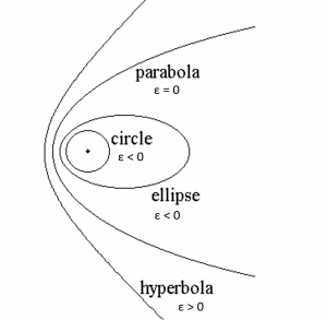
This relationship also tells us that outside the earth’s sphere of influence, since the potential energy term goes to zero, only the positive kinetic energy is left, so the overall specific mechanical energy is positive. This can only be so if the semi-major axis is negative, which in fact it is for interplanetary orbits relative to the earth. We will look at these hyperbolic trajectories later in this course.

In the next section we will put these laws together to develop the two-body equation of motion and further our understanding of orbital mechanics.

THE TWO BODY EQUATION OF MOTION

The two body equation of motion, sometimes called the restricted two-body problem, will form the basis for our understanding of orbital mechanics. In order to develop it, recall Newton’s Universal Law of Gravitation:

We defined a gravitational constant for earth-orbiting satellites as:

So, Newton’s Universal Law of Gravitation for an object around the earth becomes:

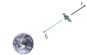
Let us take a closer look. Assume there are only two bodies involved, the earth and the satellite, and that gravity is the only force acting on the bodies. The position vector, measured from the center of the earth to the satellite, gives us this scenario:

Now using Newton’s second law and assuming both the earth and the satellite have constant masses,

Rearranging and dividing by the mass of the satellite, m_s, yields the Two-Body Equation of Motion:

where and R is the magnitude of the position vector, so,

The Two Body Equation of Motion takes the form:

Notice the assumptions that we made along the way:

1. In order to apply Newton’s Laws in the first place, our coordinate frame must be sufficiently inertial. We will consider more about coordinate systems in the next chapter.
2. The force of Earth’s gravity is the only force acting on the satellite.
3. To use Newton’s Second Law, we must assume the mass of the satellite (and the earth’s) is not changing.
4. The earth is spherically symmetrical with uniform density.
5. The mass of the earth is much greater than the mass of the satellite.
6. There are only two bodies.

Notice the two body equation of motion is a second order non-linear vector differential equation. In the next (optional) section, we will numerically integrate this equation of motion to show that the solution is a conic section. However, there is an analytical form of the solution we can find in terms of polar coordinates. For a complete derivation of this expression, see Bate (1971).

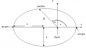
for 0 < e < 1.   Now let us consider this geometry.

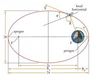
Semi-major axis

a = semi-major axis (km)

R_a = Radius to apogee (km)

R_p = Radius to perigee (km)

= specific mechanical energy (km²/s²)

For the four conic sections we will consider, these are the values for the semi-major axis

Circle:  a = R

Ellipse:  a > 0

Parabola:  a = ∞

Hyperbola:  a < 0

Eccentricity

e = eccentricity (unitless)

e = c/a

c = distance between focal points of ellipse

For the four conic sections we will consider, these are the values for eccentricity

circle: e = 0

ellipse 0 < e < 1

parabola e = 1

hyperbola e > 1

True Anomaly

=true anomaly (degrees)

True anomaly is the angle between perigee and the position vector to the satellite. We will find out soon that the eccentricity vector always points toward perigee of an orbit.

If we know the semi-major axis and eccentricity for an orbit, we can also determine expressions for R_p and R_a using the solution to the two-body equation of motion. For example, for radius of perigee:

At perigee, or a true anomaly = 0 and by expanding the numerator, this expression becomes:

R_p = a(1-e)

At apogee, or a true anomaly = 180 and by expanding the numerator, this expression becomes:

R_a = a(1+e)

CHECK YOUR UNDERSTANDING

 NUMERICAL INTEGRATION OF THE TWO BODY EQUATION OF MOTION 

We know, because it was derived by others, that the solution to the two-body equation of motion is a conic section. How do we know that? You can go through the detailed derivations found in Sellers, Bate, or some of the other references, but it will be much more valuable to prove it to yourself. You are encouraged to do this using two different methods:

1. Euler’s Integration Method.
2. Matlab’s ODE45 function (or equivalent in another programming language).

Method 1:  Euler’s Integration Method

Euler’s integration method is actually the truncated version of a Taylor series expansion. A Taylor series is a series expansion of a function about a point. A one-dimensional Taylor series is an expansion of a real function f(x) about a point, x = a, and is given by:

Where f⁽ⁿ⁾(a) is the n^th derivate of f(x) evaluated at point x = a. If a = 0, the expansion is known as the Maclaurin series and what we will use for Euler’s method (Mathworld).

If we take (x-a) as our step size, h, this expansion becomes:

Euler’s method truncates this series at:

This truncation is valid under two conditions:

1. h is small (<< 1).
2. The derivative of x is known.

Method 2:  Matlab’s ODE45 Method

ODE45 is a built-in function in Matlab that numerically integrates first order differential equations. The format is:

ODE45(ODEFUN, TSPAN, y_o)

where ODEFUN = f(t,y)

For more information on Matlab’s ODE45 function, see ODEFUN and for a general reference on Matlab see Houcque.

2 Body Equation of Motion and Initial Conditions

Given an orbit’s semi-major, a, and eccentricity, e, for any elliptical orbit, integrate the two-body equation of motion and determine it’s shape. Recall the two body equation of motion is:

This can be solved for the acceleration vector to yield:Recall the parameters associated with an elliptical orbit. We will use these parameters to establish a coordinate system and integrate this second order nonlinear differential equation.

Note in this case we have two equations that each require two initial conditions:

1.   with initial conditions:  x(0) and
2. with initial conditions:  y(0) and

If we conveniently start our integration at perigee, these initial conditions become:

x(0) = R_p = a(1-e) :  Radius at perigee

=0

y(0) = 0

= V_p :  Velocity at perigee

Finding V_p takes some explanation.

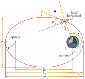
If we call the angle between the position and velocity vectors, we know

so the magnitude of is

h = RVsin

At perigee, = so

h = R_pV_p

so

Where:

For details on this derivation see Sellers Appendix C.

In this chapter, we have considered some of the important contributors to the field of astrodynamics. We have combined several of their important laws to develop the two-body equation of motion and discussed its solution. Finally, we looked at two constants of motion for orbits, the specific angular moment and specific mechanical energy, and investigated how these parameters affect satellites in orbit. In the next chapter, we will begin investigating the different types of orbits — circular, elliptical, parabolic, and hyperbolic.

Powerpoint Slides

Math Review

Ch 1 – Basic Laws – Early Astronomers and Keplers Laws

Ch 1 – Basic Laws – Newton’s Laws

Ch 1 – Basic Laws – Conservation Laws

Ch 1 – 2 Body Equation of Motion

References:

Bate, R. R., Mueller, D. D., White, J. E., & Saylor, W. W. (1971). Fundamentals of astrodynamics. Mineola (N.Y.): Dover Publications.

Difference between Heliocentric and Geocentric Models of the Universe. (2017). http://www.actforlibraries.org/wp-content/uploads/geocentric-vs-heliocentric-01.jpg

Famous Mathematicians from Germany. (2019, Jun 14). https://www.ranker.com/list/famous-mathematicians-from-germany/reference

Giphy. (2019, September 06). Motion Sun GIF – Find & Share on GIPHY. https://giphy.com/gifs/planet-closer-slice-pRqK2YcBYQp0s

Greek City Times. (2018, May 21). Why Ancient Greek Philosophers Are the Greatest Thinkers to Have Graced This Earth.  https://greekcitytimes.com/2018/05/15/why-ancient-greek-philosophers-are-the-greatest-thinkers-to-have-graced-this-earth/

Houcque, D. (2005, August). INTRODUCTION TO MATLAB FOR ENGINEERING STUDENTS. https://moodle2.units.it/pluginfile.php/256936/mod_resource/content/1/introduction-to-matlab_2018.pdf

Lowensohn, J. (2014, August 23). SpaceX Falcon 9 test vehicle explodes during ‘particularly complex’ Texas test flight. https://www.theverge.com/2014/8/22/6058469/spacex-falcon-9-rocket-explodes-during-texas-test-flight

Taylor Series. (2021, January 11).  https://mathworld.wolfram.com/TaylorSeries.html

Mathematical Treasure: Newton’s Principia. (n.d.). Retrieved January 25, 2021, from https://www.maa.org/press/periodicals/convergence/mathematical-treasure-newtons-principia

Minute and second of arc. (2020, December 28). Retrieved January 22, 2021, from https://en.wikipedia.org/wiki/Minute_and_second_of_arc

Newton’s Law of Universal Gravitation. (2021). https://www.physicsclassroom.com/class/circles/Lesson-3/Newton-s-Law-of-Universal-Gravitation

Odefun. (2021). https://www.mathworks.com/help/matlab/ref/ode45.html

Randolph, K. (2017, April 17). Tycho Brahe Rock Star of His Day. https://www.slideshare.net/KellaRandolph/tycho-brahe-rock-star-of-his-day

Rocket Thrust. (2014, June 12). https://www.grc.nasa.gov/WWW/k-12/rocket/rktth1.html

Sellers, Jerry Jon.  (2005).  Understanding Space:  An Introduction to Astronautics, 3rd edition.  McGraw-Hill.

Solpass. (2013). Potential and Kinetic Energy. https://www.solpass.org/science6-8-new/standards/standard_ps6.html

Tycho Brahe: The Astronomer with A Drunken Moose. (2013, May 09). https://www.mentalfloss.com/article/50409/tycho-brahe-astronomer-drunken-moose