7 Chapter 7 – Manuevering

Many people do not think about how how we move from one location to another in space. When watching a Hollywood movie, we might see our favorite actor just jump out of their spacecraft and float to another that is a couple hundred meters away. Unfortunately, as great as this looks on the big screen, it is not realistic. When in orbit, that almighty force of gravity is still a factor. It is what makes orbits possible, however, it is what also makes those Hollywood stunts impossible.

While in orbit, objects are constantly moving, even if they do not appear so. Thus, instead of fighting against these forces, the best course of action is to work with them. In this chapter, we will look at how we purposefully change some of the Classical Orbital Elements (COEs) of an orbit, whether it be semi-major axis, inclination, or even Right Ascension of Ascending Node (RAAN).

When it comes to changing orbits in the same plane, there are a multitude of different ways to approach the problem. What if we want to conserve fuel? What if we want to change orbits as quickly as possible? All of these questions and more are going to be answered in this chapter.

HOHMANN TRANSFER 

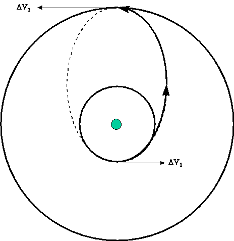
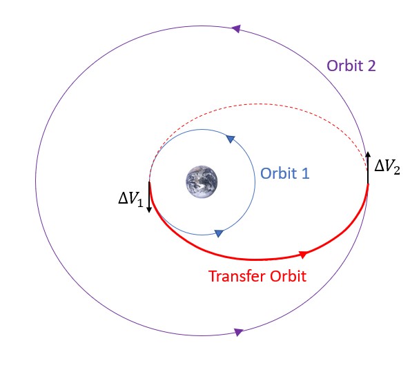
The first type of maneuver we are going to look at is called a Hohmann Transfer, which is the most fuel-efficient maneuver for satellites in coplanar orbits (i.e. in the same orbital plane). The goal of a Hohmann Transfer is to transfer from one orbit to another. Usually this is from a smaller orbit to a larger one, but it could also be in the other direction. Both maneuvers are achieved by moving into an elliptical transfer orbit. A huge advantage of this type of transfer is that it only requires two energy boosts that we call Delta Vs , ΔVs, or velocity burns. This maneuver requires the need to burn once to get from the initial orbit to the transfer orbit and then again to get from the transfer orbit to the final orbit. The general format of this can be seen in Figure 1:

There are a few assumptions that need to be made in order to perform the necessary calculations for this maneuver. They include:

1) Orbits are co-planar

2) Orbits are co-apsidal

3) Tangential burns

4) Instantaneous burns

These assumptions are each described in more detail below.

1) CO-PLANAR

One of the most important assumptions is that the initial and final orbits are co-planar. This means that the two orbits have the same inclination and RAAN. Try to picture a satellite in orbit on a piece of paper (i.e., in a 2-dimensional frame).  Not considering perturbations, which will be discussed later, the satellite would not leave the paper. The initial and final orbits would have to be on the same piece of paper. If the initial orbit was on the paper and the final orbit was not, they would not be coplanar. If the two orbits are not coplanar, this algorithm will not work.

2) CO-APSIDAL

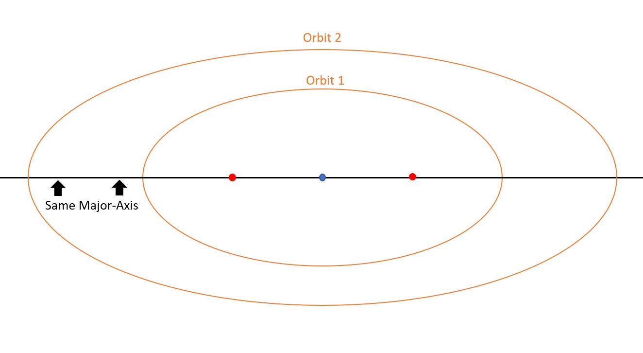
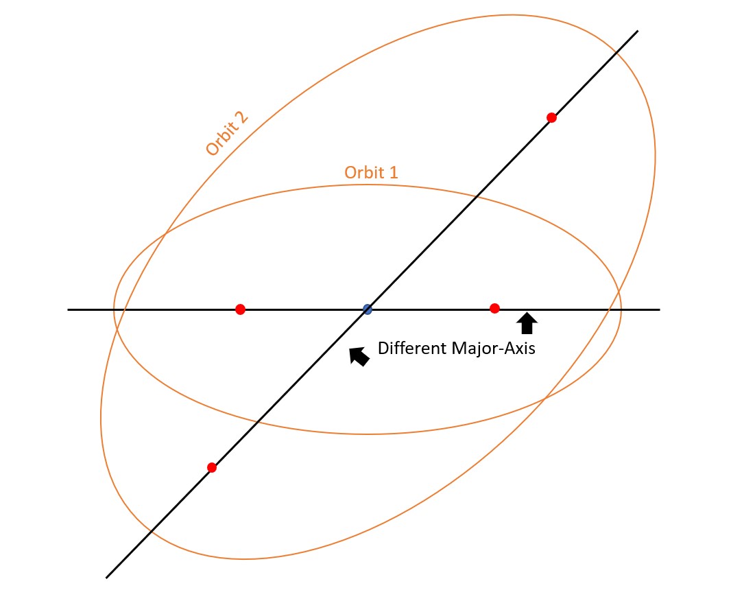
The second assumption that needs to be made is that the first and final orbits are co-apsidal. For circular orbits, this means that the centers of the orbits need to be aligned. For elliptical orbits, this means that their major axes must be aligned. This can be seen in Figure 2 and Figure 3:

Co-apsidal:

Not Co-apsidal:

3) TANGENTIAL BURNS

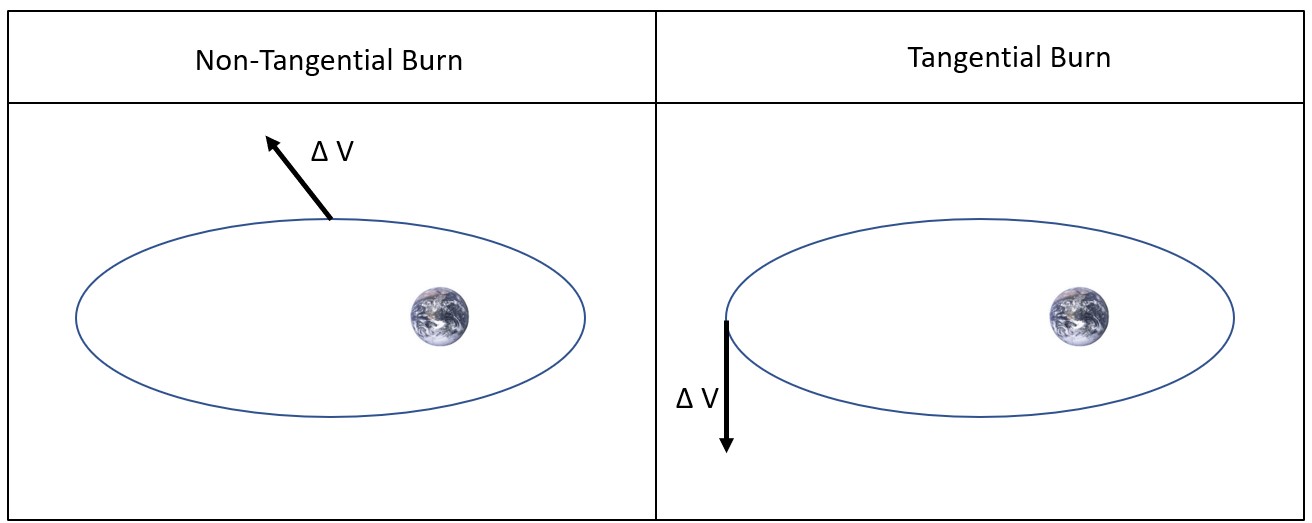
We also assume that velocity burns are tangent to the orbit and parallel to the velocity vector at that point. This means that when burning, it should not be performed in a direction other than along the line of the velocity vector. In other words, the velocity burn should be parallel to the direction that the velocity is already going in, which is shown in the image below. If the velocity burn is not done in this way, then it is not the most efficient velocity change and, therefore, is not a Hohmann Transfer. This is shown in Figure 4:

4) INSTANTANEOUS BURNS

Instantaneous burns are more of an ideal assumption. It describes an instantaneous change in velocity between two orbits, which is not realistic in any way. It is impossible in our universe for something to change between two completely different velocities in an instant. However, for a Hohmann Transfer, we assume that it is because the small 2-5 minute burn is small when compared to the much longer time for the transfer.

We are first going to go through the algorithm from a smaller circular orbit to a larger circular orbit (Figure 5), then we will discuss how to perform this maneuver (Figure 6) with two elliptical orbits.

CIRCULAR TO CIRCULAR

The transfer orbit, as discussed before, is an elliptical orbit. This orbit is going to be traveled from perigee to apogee, i.e., only 180°, or half of its full period. The transfer orbit’s semi-major axis is half of the sum of the radii of the initial and final orbits can be solved with Equation 1:

(1)

[latex]\large a_t=\frac{R_1+R_2}{2}[/latex]

The key to the remainder of the Hohmann Transfer algorithm is keeping close track of the velocities. First, let us find the satellite’s velocity in the initial orbit. Remember, at this point we are assuming the initial and final orbits are circular. Because of this, the velocity is equal to Equation 2:

(2)

[latex]\large V_1=\sqrt{\frac{\mu}{R_1}}[/latex]

The next step is to calculate the specific mechanical energy of the transfer orbit. We are going to use the form of the equation with semi-major axis, a, because we easily calculated the transfer orbit earlier. So, we can now use that here with Equation 3:

(3)

[latex]\large \varepsilon_t=-\frac{\mu}{2 a_t}[/latex]

Remember that there is another equation for specific mechanical energy that uses velocity and position. We are going to use Equation 4 for the transfer orbit:

(4)

[latex]\large \varepsilon_t=\frac{V^2}{2}-\frac{\mu}{R}[/latex]

So here, we can use ε_t and rearrange it to solve for velocity, using R₁ for the radius, to determine the velocity at perigee of the transfer orbit by using Equation 5—just when it leaves the initial orbit and enters into the transfer orbit.

(5)

[latex]\large V_{t 1}=\sqrt{2\left(\frac{\mu}{R_1}+\varepsilon_t\right)}[/latex]

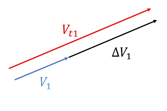
We now have the velocity of the satellite at the same moment of two different orbits (our initial orbit and transfer orbit). With both of these, we can calculate the burn velocity, ΔV, that is required to “move” the object from the initial orbit to the transfer orbit. It is as simple as taking the absolute value of the difference between these two velocities with Equation 6:

(6)

[latex]\large \Delta V_1=\left|V_{t 1}-V_1\right|[/latex]

Sometimes, it can help to visualize these vectors. If you direct your attention to the graphic below (Figure 7), you will see a figure of these velocities. In this case, V_t1 is larger than V₁, therefore ΔV is going to be the difference between these.

Now, we have just moved from the initial orbit to the transfer orbit. We are then going to travel this orbit until apogee is reached, where we are then going to move to the final orbit. This is a very similar process as going from the initial orbit to the transfer orbit.

We first need to calculate the velocity of the final orbit with Equation 7. Again, note that since we are assuming a circular orbit, speed is equal at all locations.

(7)

[latex]\large V_2=\sqrt{\frac{\mu}{R_2}}[/latex]

We then find the velocity the object is traveling at the apogee of the transfer orbit using the specific mechanical energy of the transfer orbit, which is shown through Equation 8:

(8)

[latex]\large V_{t 2}=\sqrt{2\left(\frac{\mu}{R_2}+\varepsilon_t\right)}[/latex]

We can now use these two velocities in equation (9) to find the magnitude of the burn needed to maneuver from the transfer orbit into the final orbit:

(9)

[latex]\large \Delta V_2=\left|V_2-V_{t 2}\right|[/latex]

It is also important to know the total amount of burn it will take to complete a Hohmann Transfer, as we need to know the amount of fuel it will take to complete it. We do this by summing the two burn velocities we have calculated and entering them into Equation 10:

(10)

[latex]\large \Delta V_{\text {total }}=\Delta V_1+\Delta V_2[/latex]

Another piece of information that is important to calculate is the time of flight, TOF, of this orbit. Since we know it is half of the period of the orbit, we can calculate the following with either TOF Equations (11):

(11)

[latex]\large T O F=\frac{1}{2}\left(2 \pi \sqrt{\frac{a_t^3}{\mu}}\right)[/latex]

or

[latex]\large T O F=\pi \sqrt{\frac{a_t^3}{\mu}}[/latex]

Here is a link to an algorithm for a Hohmann Transfer:  George_Hohmann Transfer Algorithm

For additional information on the Hohmann Transfer, watch the following simulation in Video 1 of a transfer from a smaller to a larger orbit.

_{Video 1: Simulation of Hoffman Transfer (George, 2021)}

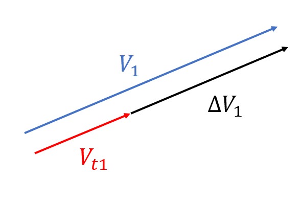
When considering maneuvering from a large orbit to a small orbit by using a Hohmann Transfer, the process is essentially the same. The same algorithm applies, however there is a small change. We are going to perform a retro burn (anti-velocity burn), which is shown in Figure 8. Do not get scared by the verbiage. All this means is that we are going to have to slow down (burn opposite to current velocity direction) instead of speed up. This is because now, our V₁ velocity is going to be larger than the V_t1 velocity as pictured in the image below. If you were wondering why we use absolute values in our burn calculations, this is why. If we did not do this, we would get a negative speed, which is not possible in this scenario.

Below is a simulation of a Hohmann Transfer from a larger to a smaller orbit.

EXAMPLE 1

A satellite in a higher circular orbit at R = 6878 km needs to transfer to a smaller orbit at R = 6528 km in order to meet a new payload requirement.

Find the total Delta V required for a Hohmann Transfer and the time of flight the transfer will take.

ELLIPTICAL TO ELLIPTICAL

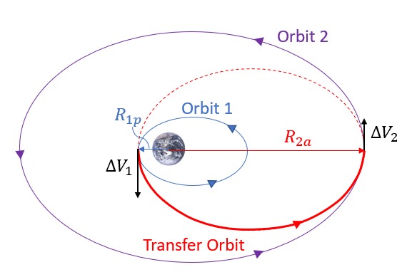
With the knowledge that no orbit is perfectly circular in reality, we are mostly going to be dealing with elliptical orbits (Figure 9). So, let us apply this to Hohmann Transfers as well (Figure 10). In truth, there is not going to be much difference between both orbits, circular to circular and/or elliptical to elliptical. The first step to keep in mind is assumption. In particular, the assumption that the major axes must be aligned (co-apsidal) must be true, as this is extremely important for Hohmann Transfers performed between elliptical orbits.

The second step is to pay attention to the velocities, which is the key to Hohmann Transfers. We are trying to make this as fuel-efficient as possible; in other words, we want our total burn (ΔV_total) to be as small as possible. When performing a Hohmann Transfer from a smaller to a larger orbit, the object enters the transfer orbit at perigee and exits at apogee. Since we always need to increase the speed of the spacecraft to get it into this orbit, we would need to increase the speed as little as possible in order to keep the magnitude of that burn low. To achieve this, we are going to begin the transfer at the perigee of the first orbit. This is because at perigee, the object in orbit is moving faster than at any other point. Therefore, it is going to take the least amount of energy than any other point to get it into its transfer orbit. Naturally, this means that it is going to exit the transfer orbit and enter at apogee of the second orbit.

When going through the algorithm, the first big difference is at the beginning. Unlike circular orbits, we cannot simply take half of the sum of the radii of the initial and final orbits. This is because the R vector is always changing in elliptical orbits so, as discussed previously, we have to pay attention to where we are entering and exiting the transfer orbit. Because we are going to leave the first orbit at perigee and enter the final orbit at apogee, we can use those two radii to sum.

Recall Equation 12 for radius of perigee is:

(12)

[latex]\large R_p=a(1-e)[/latex]

Also note the Equation 13 for radius of apogee is:

(13)

[latex]\large R_a=a(1+e)[/latex]

If only given semi-major axis and eccentricity, we can substitute the known values for that into  Equation 14:

(14)

[latex]\large a_t=\frac{R_{1 p}+R_{2 a}}{2}=\frac{a_1\left(1-e_1\right)+a_2\left(1+e_2\right)}{2}[/latex]

The next step of this process is determining the velocity of the satellite before it performs the burn in orbit one. For this, we are going to use equation (15) for velocity:

(15)

[latex]\large V=\sqrt{2\left(\frac{\mu}{R}+\varepsilon\right)}[/latex]

In order to solve this equation, you need to use equation (16) to solve for specific mechanical energy of orbit one.

(16)

[latex]\large \varepsilon_1=-\frac{\mu}{2 a_1}[/latex]

This value can then be used to determine the velocity at perigee of the initial orbit by rearranging the other equation for specific mechanical energy as seen in Equation 17:

(17)

[latex]\large V_1=\sqrt{2\left(\frac{\mu}{R_{1 p}}+\varepsilon_1\right)}[/latex]

Just like from circular to circular, the next step is to calculate the specific mechanical energy of the transfer orbit. We are going to use the equation with semi-major axis, a, because we easily calculated that of the transfer orbit earlier. So, we can now use that here in Equation 18:

(18)

[latex]\large \varepsilon_t=-\frac{\mu}{2 a_t}[/latex]

The equation for the velocity of the transfer orbit as it enters the second orbit is going to look very similar to the one we just calculated for perigee at the first orbit, but notice that we use a different specific mechanical energy. However, R is still going to be the same in Equation 19:

(19)

[latex]\large V_{t 1}=\sqrt{2\left(\frac{\mu}{R_{1 p}}+\varepsilon_t\right)}[/latex]

The burn velocity in equation (20) still remains the difference between the two velocities:

(20)

[latex]\large \Delta V_1=\left|V_{t 1}-V_1\right|[/latex]

After traveling halfway around the transfer orbit, we are at the position to maneuver into the final orbit. So, let us first determine how fast we are going to need to be traveling. For our velocity equation, since we are in an elliptical orbit, we first need to identify specific mechanical energy by using Equation 21:

(21)

[latex]\large \varepsilon_2=-\frac{\mu}{2 a_2}[/latex]

Then we can solve for velocity at our final obit. Remember, we are entering this final orbit at its apogee, so be sure to use the radius of apogee, R_a, in your calculations in Equation 22:

(22)

[latex]\large V_2=\sqrt{2\left(\frac{\mu}{R_{2 a}}+\varepsilon_2\right)}[/latex]

We then find the velocity the object is going to be traveling at the apogee of the transfer orbit using, again, the specific mechanical energy of the transfer orbit in Equation 23:

(23)

[latex]\large V_{t 2}=\sqrt{2\left(\frac{\mu}{R_{2 a}}+\varepsilon_t\right)}[/latex]

We can now use these two velocities to find the burn between the transfer orbit and the final orbit by inserting them into Equation 24:

(24)

[latex]\large \Delta V_2=\left|V_2-V_{t 2}\right|[/latex]

It is still important to calculate the total change in velocity, which we use the same equation as before, which is represented in Equation 25:

(25)

[latex]\large \Delta V_{\text {total }}=\Delta V_1+\Delta V_2[/latex]

This also goes for time of flight in Equation 26:

(26)

[latex]\large T O F=\frac{1}{2}\left(2 \pi \sqrt{\frac{a_t^3}{\mu}}\right)[/latex]

or

[latex]\large T O F=\pi \sqrt{\frac{a_t^3}{\mu}}[/latex]

EXAMPLE 2

A satellite is in an elliptical orbit with a semi-major axis, a = 8,650 km, and an eccentricity, e = 0.3. It needs to be transferred to an orbit with a semi-major axis, a = 15,235 km, and an eccentricity, e = 0.4. Find the ΔV and time of flight required to perform this maneuver.

SIMPLE PLANE CHANGE

Another type of maneuver we can perform is changing only the tilt or swivel of an orbit. We call this a Simple plane change. This changes one of two COE’s: inclination, i, or RAAN, Ω, as these are the two COE’s that deal with the tilt and swivel of an orbit.

So, if we had a satellite or other object in orbit and we had to maneuver it to another orbit with all the same COE’s except inclination or RAAN, we would perform a Simple plane change. This would be the case for Case One of launch windows where inclination was less than the launch site latitude. If you remember, we could not launch it directly into orbit. Unfortunately, we are sometimes confined to certain inclinations and can only launch from a specific location that has a latitude greater than the inclination. Luckily, we do not have to fret as it would still be possible to get into our desired orbit with the help of a simple plane change!

Let us begin by considering the general form of this maneuver. As stated previously, the ONLY thing that would change in this type of maneuver is inclination or RAAN. This means that the magnitudes of the initial and final velocities are the same. With this information, we can make an equilateral triangle where the third side is the burn velocity (Figure 11):

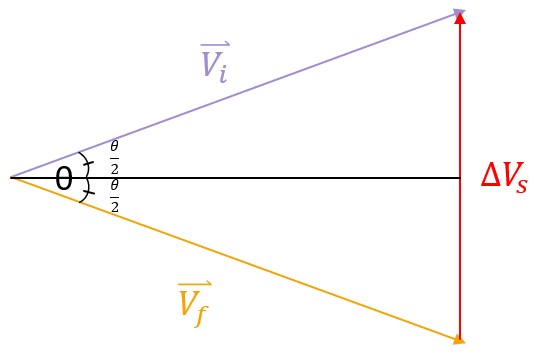
Using a little trigonometry for one of the right triangles in Equation 27:

(27)

[latex]\large\sin \frac{\theta}{2}=\frac{\frac{\Delta V_s}{2}}{V_i}[/latex]

Now, we can rearrange this equation to solve for the burn velocity, giving us Equation 28:

(28)

[latex]\large\Delta V_s=2 V_i \sin \left(\frac{\theta}{2}\right)[/latex]

Notice that the Delta V is directly proportional to the velocity of the satellite in the orbit, so it is prudent to perform plane change maneuvers as far away from the earth as possible.

CHANGING INCLINATION

Now that we have the general form of the equation, let us consider each case. The first is a change in inclination. The important step with this is that the maneuver can only be performed over the ascending or descending node. This is because the line that connects these nodes is what the orbit tilt, or inclination, rotates about. For the equation (29), we are going to use the generic equation from above where θ = Δi:

(29)

[latex]\large\begin{gathered} \Delta V_s=2 V_i \sin \left(\frac{\theta}{2}\right) \\ \theta=\Delta i \end{gathered}[/latex]

Below is a simulation of a Simple plane change for inclination (Video 3). Notice the maneuver is performed at the ascending node.

Video 3: Simple Plane Change Inclination (George, 2023)

CHANGING RAAN

Changing RAAN is very similar. Much like how the Simple plane change has to be performed over the ascending or descending node for inclination, a Simple plane change of only RAAN can only be performed above the North or South Pole because the orbital swivel, or RAAN, rotates about the line connecting the poles, or the Earth’s axis of rotation. The only change in the generic equation is that θ = ΔΩ in Equation 30:

(30)

[latex]\large\begin{gathered} \Delta V_s=2 V_i \sin \left(\frac{\theta}{2}\right) \\ \theta=\Delta \Omega \end{gathered}[/latex]

Below is a simulation of a Simple plane change for RAAN (Video 4). Notice the maneuver is performed over the North Pole.

Video 4: Simple Plane Change (George, 2023)

EXAMPLE 3

A satellite in a circular orbit with a speed of 8 km/s needs to maneuver from an orbit at an inclination of 32.3˚ to 72.3˚.  How much ΔV is required?

COMBINED PLANE CHANGE

In addition to the Hohmann Transfer and Simple plane change, there is also a maneuver called a Combined plane change. Unlike the Simple plane change, where only the direction of velocity is changed but the magnitude remains unchanged, both the direction and magnitude of velocity is changed for a Combined Plane Change. This allows for an orbit to change from one size orbit (smaller or bigger) to another size, as well as changing the inclination or RAAN of the orbit. With the methods presented thus far, this maneuver could be completed with the two burns of a Hohmann Transfer and followed by a Simple plane change, which requires three burns. Unfortunately, this is not very fuel-efficient. What would make this process as fuel-efficient as possible would be combining one of those Hohmann burns with the Simple plane change burn, thus reducing the total number of burns down to two. This method is called a Combined plane change and can be seen in Video 5 below:

Video 5: Combined Plane Change (George, 2023)

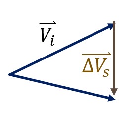
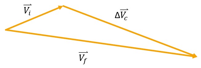
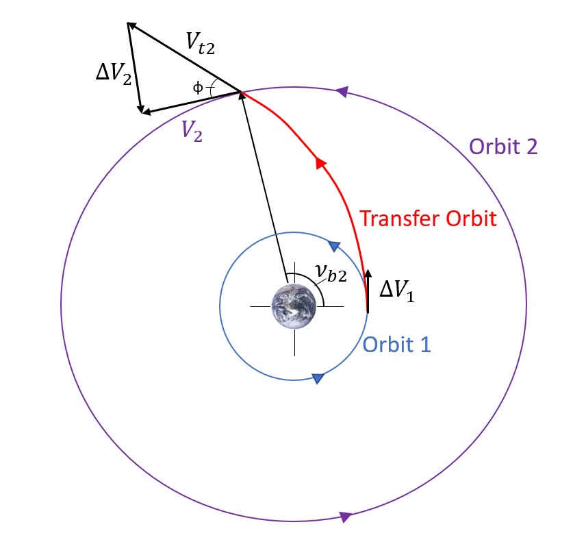
To start to understand this maneuver, let us draw the velocities of this out and perform a little vector algebra (Figure 12). We are going to focus on the combined burn instead of the first or second Hohmann burn, as you should already have the tools to determine that burn.

Let us first look at the Simple plane change aspect where is the initial velocity and is the Simple plane change burn velocity. The third vector will see points in the direction of the final velocity, but does not have the new magnitude, so we are going to keep it unnamed for now.

Next, let us add the Hohmann burn to the mix (Figure 13). Try to think of it as adding to the “final” velocity of the Simple plane change (not the initial). We are going to label this . The vector between the tails of the initial velocity and the second Hohmann Transfer burn velocity is going to be the burn of this combined plane change, labeled .

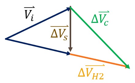
On a side note, if you needed proof that this method is cheaper than performing a full Hohmann Transfer and then performing a Simple plane change, let us look at the triangle that combines all of these sides. If we recall the identity from geometry, that the sum of the two shorter sides of a triangle is greater than the longer side, we can see that no matter what, the burn of the combined plane change is going to be less than the sum of the Simple plane change burn and the second Hohmann Transfer burn. In mathematical terms, Equation 31:

(31)

[latex]\large V_c<\Delta V_s+\Delta V_{H 2}[/latex]

Combining all of this together and eliminating some unnecessary vectors, we are left with the following vector addition (Figure 14):

Using the law of cosines to get an equation almost solving for the combined burn, we get Equation 32:

(32)

[latex]\large\Delta V_c^2=V_i^2+V_f^2-2 V_i V_f \cos \theta[/latex]

Now, taking the square root of both sides, the generic form for the combined plane change equation (33) is:

(33)

[latex]\large\Delta V_c=\sqrt{V_i^2+V_f^2-2 V_i V_f \cos \theta}[/latex]

Again, exactly like the Simple plane change, theta is dependent on what COE is being changed to, either inclination or RAAN. The change in either one can be used as theta in the equation (34):

(34)

[latex]\large \theta=\Delta i[/latex]

Or

[latex]\large \theta=\Delta \Omega[/latex]

Just like the Simple plane change, the maneuver must be performed above the equator for inclination and above the north or south pole for RAAN.

With this generic equation, we can split the combined plane change into two cases: moving from a smaller orbit to a larger orbit and moving from a larger orbit to a smaller orbit.

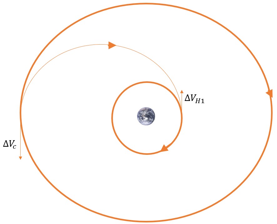
CASE ONE: SMALLER TO LARGER ORBIT

In the case of an orbit going from a smaller orbit to a larger orbit, we start with the first Hohmann burn and then perform the combined plane change at the final orbit. If it helps, when doing the first Hohmann burn, imagine going to an orbit of the size of the final orbit, yet it is in the same plane (Figure 15). This is because the transfer orbit is going to be bringing it to the point of the combined burn which will be in the same plane as the initial orbit. We get Equation 35:

(35)

[latex]\large\text { a) } \Delta V_{H 1}=\left|V_{t 1}-V_1\right|[/latex]

The second step is performing the combined plane change. Let us use the generic equation (36) and define some of the variables:

(36)

[latex]\large \text { b) } \Delta V_c=\sqrt{V_i^2+V_f^2-2 V_i V_f \cos \theta}[/latex]

where

[latex]\large V_i=V_{t 2}[/latex]

[latex]\large V_f=V_2[/latex]

The final step is to use equation (37) to find the total burn it would take to do this entire maneuver, which is just the sum of the two burns.

(37)

[latex]\large\text { c) } \Delta V_{\text {total }}=\Delta V_{H 1}+\Delta V_c[/latex]

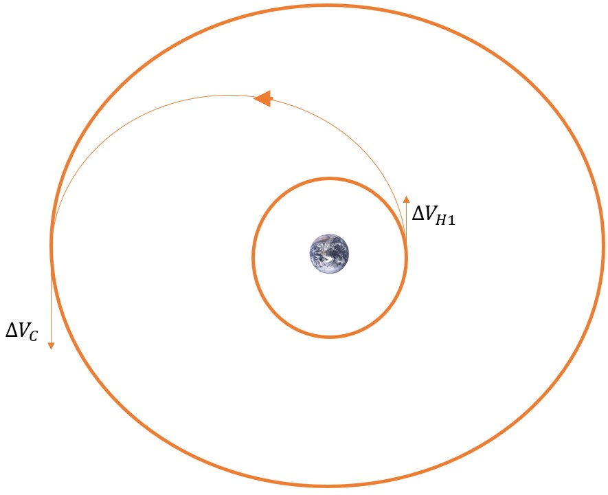
CASE TWO: LARGER TO SMALLER ORBIT

This case follows a very similar process to Case One except it is performed in reverse order. First, the combined plane change is performed followed by the second Hohmann burn in the final orbit. You can see a two-dimensional view of this process in Figure 16:

Now, Step A is performing the combined plane change in Equation 38:

(38)

[latex]\large\text { a) } \Delta V_c=\sqrt{V_i^2+V_f^2-2 V_i V_f \cos \theta}[/latex]

where

[latex]\large V_i=V_1[/latex]

[latex]\large V_f=V_{t 1}[/latex]

This maneuver is followed by the second Hohmann burn to get into the correctly sized orbit (equation 39):

(39)

[latex]\large\text { b) } \quad \Delta V_{H 2}=\left|V_{t 2}-V_2\right|[/latex]

When adding both of these together, we end with the total burn (equation 40):

(40)

[latex]\large\text { c) } \Delta V_{\text {total }}=\Delta V_c+\Delta V_{H 2}[/latex]

EXAMPLE 4

A satellite is in a circular orbit with a radius of 6570 km and an inclination of 28°. It needs to be moved to a circular orbit with a radius of 42,160 km and an inclination of 0°.  This scenario could be a satellite launched from Cape Canaveral in Florida headed for a geostationary orbit.

Find the total burn using the most fuel-efficient transfer.

BI-ELLIPTICAL

Another type of transfer between two coplanar orbits is called a bi-elliptical orbit. As the name implies, it uses two elliptical transfer orbits in series to transfer the object from one orbit to another. This can be a little difficult to visualize, so direct your attention to this simulation (Video 6) for clarity:

Video 6: Bielliptic (George, 2023)

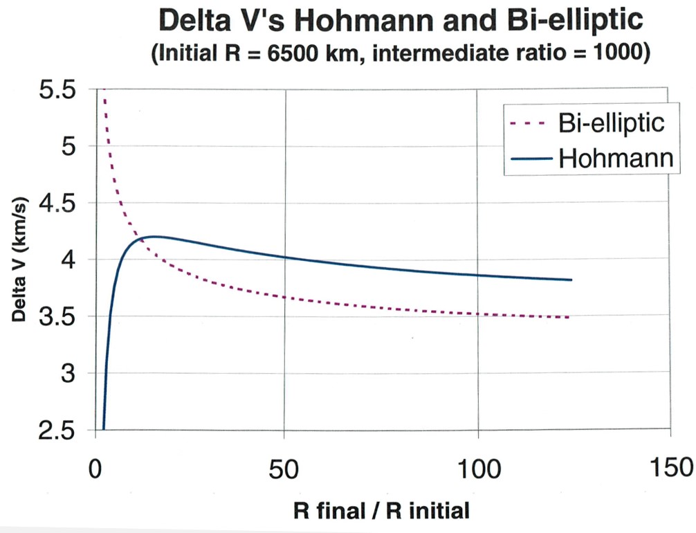
A valid question to ask when looking at this maneuver is, “Why would we do this and take longer when we can just use a Hohmann Transfer?” That is an excellent question! While it is true that a bi-elliptic transfer will always take a longer amount of time than a Hohmann Transfer, unfortunately, sometimes time is not the issue. Energy, in other words, fuel, is also an important factor in deciding what kind of transfer to perform. For smaller transfers, Hohmann Transfers are almost always the route to take as they are not only quicker, but also more energy effective than a bi-elliptic transfer. But over a certain distance ratio, the bi-elliptic transfer becomes more fuel-efficient than the Hohmann Transfer, as seen in Figure 17 below. If time is less of a priority in these cases, a bi-elliptic transfer might be more beneficial.

Now, let us take a look at the process of completing a bi-elliptical transfer (Figure 18). First, we should define all the orbits and burns we are going to label (Figure 19):

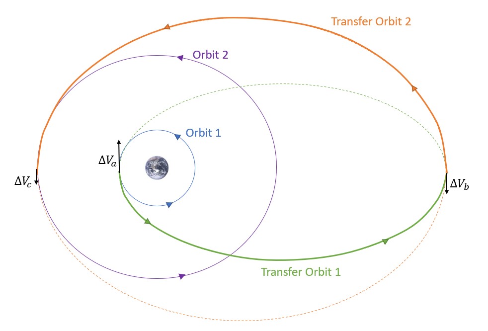
The first step in this process is determining the semi-major axis of the first transfer orbit. This is the orbit shown above in green. Recalling the equation using half of the sum of radius of perigee and radius of apogee, we can determine a_t1. Just like the Hohmann Transfer, the radius of perigee of this orbit is equal to the radius of the first orbit. The radius of apogee is a different story. This radius for the first transfer orbit is defined somewhere beyond the radius of the final orbit. We are going to call the distance from the center of the Earth to this point, Rb. It is up to the person creating this transfer to define what this distance is. See Equation 41:

(41)

[latex]\large a_{t 1}=\frac{R_1+R_b}{2}[/latex]

Using this result, we can find the specific mechanical energy of this first transfer orbit with Equation 42.

(42)

[latex]\large\varepsilon_{t 1}=-\frac{\mu}{2 a_{t 1}}[/latex]

The next step is determining the velocity of the initial orbit which is given by Equation 43:

(43)

[latex]\large V_1=\sqrt{\frac{\mu}{R_1}}[/latex]

We also need the velocity of the transfer orbit initially. We are going to define this as point a, giving us a velocity of Equation 44:

(44)

[latex]\large V_{t 1 a}=\sqrt{2\left(\frac{\mu}{R_1}+\varepsilon_{t 1}\right)}[/latex]

Finally, for this initial burn, we just need to find the absolute value of the difference between the velocities with Equation 45 to know how much energy will be needed to enter the first transfer orbit.

(45)

[latex]\large\Delta V_a=\left|V_{t 1 a}-V_1\right|[/latex]

The next step (46) is where the bi-elliptical transfer truly differs from the Hohmann Transfer. When at apogee of the first transfer orbit, we are ready to transfer to the second transfer orbit. First, while in the first transfer orbit, we can determine what the velocity will be at this point.

(46)

[latex]\large V_{t 1 b}=\sqrt{2\left(\frac{\mu}{R_b}+\varepsilon_{t 1}\right)}[/latex]

Next, we need to define some parameters for the second transfer orbit. The process will be very similar to the first. The radius of apogee remains the same at a distance of R_b from the Earth. The radius of perigee, on the other hand, will be our final orbit. So, it will have a radius of R₂. This gives us Equation 47:

(47)

[latex]\large a_{t 2}=\frac{R_b+R_2}{2}[/latex]

Again, we can find the specific mechanical energy of this orbit with Equation 48:

(48)

[latex]\large\varepsilon_{t 2}=-\frac{\mu}{2 a_{t 2}}[/latex]

Before we work on the final burn, remember, at this point in the process we are still at point b. So, let us determine the velocity at this point of the second transfer orbit with Equation 49:

(49)

[latex]\large V_{t 2 b}=\sqrt{2\left(\frac{\mu}{R_b}+\varepsilon_{t 2}\right)}[/latex]

Now that we have both velocities at point b, we can take the difference to determine the burn with Equation 50:

(50)

[latex]\large\Delta V_b=\left|V_{t 2 b}-V_{t 1 b}\right|[/latex]

Our final point of interest is where the second transfer orbit and the final orbit intersect. We are going to call this point c. In order to determine the final burn, we first need the velocity of the second transfer orbit at that point using Equation 51:

(51)

[latex]\large V_{t 2 c}=\sqrt{2\left(\frac{\mu}{R_2}+\varepsilon_{t 2}\right)}[/latex]

We also need the final velocity of the final orbit which can be more simply found with Equation 52:

(52)

[latex]\large V_2=\sqrt{\frac{\mu}{R_2}}[/latex]

With both of these velocities, the burn at point c can be found by taking the absolute difference with Equation 53:

(53)

[latex]\large\Delta V_c=\left|V_2-V_{t 2 c}\right|[/latex]

Exactly like a Hohmann Transfer, it is important to know the total burn needed to complete this maneuver. We can find this by taking the sum of every burn we have calculated up to this point with Equation 54:

(54)

[latex]\large\Delta V_{\text {total }}=\Delta V_a+\Delta V_b+\Delta V_c[/latex]

Another important piece of information that might be required is the time of flight. To determine that, we would add together in Equation 55 how long it would take to go around half of each transfer orbit since we are only going around half of each:

(55)

[latex]\large\text { TOF }=\pi \sqrt{\frac{a_{t 1}^3}{\mu}}+\pi \sqrt{\frac{a_{t 2}^3}{\mu}}[/latex]

EXAMPLE 5

An object in a circular orbit with a radius of 8230 km needs to be moved to another circular orbit with a radius of 260,000 km. It was determined by a group of NASA engineers (who looked at a very convenient graph) that the most fuel-efficient transfer for this specific maneuver is a bi-elliptical transfer with a transfer point 800,000 km away. Find the total ΔV and time of flight required for this transfer.

ONE-TANGENT MANEUVERS

Both Hohmann and bi-elliptical transfers are great and each have their advantages and disadvantages, but there also lies another option. As stated before, the bi-elliptical orbit is beneficial in saving energy, but not in time. But what if we are more concerned about time and worried less about fuel consumption? This is where one-tangent burns can be extremely beneficial.

Just like the bi-elliptical transfer, the one-tangent burn nearly explains itself. This method has one tangent burn and one non-tangent burn, as opposed to Hohmann and bi-elliptical transfers, which only use tangential burns. Another way this type of maneuver is unique is that it does not use only an elliptical transfer orbit. It can use any orbit to get from point A to point B including parabolic and hyperbolic orbits.

With this book, we are going to take a more simple look at one-tangent burn transfers and only analyze transfers between two circular orbits as seen in the following image:

The derivation for some of these equations are a little difficult. You can find the algorithm below in Equation 56, but we will not be getting too in depth into one-tangent burns.

(56)

[latex]\large\begin{gathered} e_{\text {t,perigee }}=\frac{\frac{R_1}{R_2}-1}{\cos \left(v_{t 2}\right)-\frac{R_1}{R_2}} \\ e_{\text {t,apogee }}=\frac{\frac{R_1}{R_2}-1}{\cos \left(v_{t 2}\right)+\frac{R_1}{R_2}} \end{gathered}[/latex]

Only one of these values are going to be used. It depends on the setup of the problem and orbit type (elliptic to elliptic, circular to circular, etc.). This goes for both eccentricity, e, and semi-major axis, a, as in Equation 57.

(57)

[latex]\large a_{t, \text { perigee }}=\frac{\frac{R_1}{R_2}}{1-e_{t, \text { perigee }}}[/latex]

[latex]\large a_{t, \text { apogee }}=\frac{\frac{R_1}{R_2}}{1+e_{t, \text { apogee }}}[/latex]

[latex]\large \varepsilon_t=-\frac{\mu}{2 a_t}[/latex]

E is eccentric anomaly, the same eccentric anomaly that was discussed in Chapter 6, as in the following Equation 58.

(58)

[latex]\large E=\cos ^{-1}\left(\frac{e_t+\cos \left(v_{t 2}\right)}{1+e_t \cos \left(v_{t 2}\right)}\right)[/latex]

[latex]\large \text { TOF }=\sqrt{\frac{a_t^3}{\mu}}\left[2 k \pi+\left(E-e_t \sin (e)\right)-\left(E_0-e_t \sin \left(E_0\right)\right)\right][/latex]

[latex]\large V_1=\sqrt{\frac{\mu}{R_1}}[/latex]

[latex]\large V_{t 1}=\sqrt{2\left(\frac{\mu}{R_1}+\varepsilon_t\right)}[/latex]

[latex]\large V_2=\sqrt{\frac{\mu}{R_2}}[/latex]

[latex]\large V_{t 2}=\sqrt{2\left(\frac{\mu}{R_2}+\varepsilon_t\right)}[/latex]

[latex]\large \Delta V_1=\left|V_{t 1}-V_1\right|[/latex]

[latex]\large \phi_{t 2}=\tan ^{-1}\left(\frac{e_t \sin \left(v_{t 2}\right)}{1+e_t \cos \left(v_{t 2}\right)}\right)[/latex]

[latex]\large \Delta V_2=\sqrt{V_{t 2}^2+V_2^2-2 V_{t 2} V_2 \cos \left(\phi_{t 2}\right)}[/latex]

[latex]\large \Delta V_{\text {total }}=\Delta V_1+\Delta V_2[/latex]

This process can be seen in more detail in Fundamentals of Astrodynamics and Applications by David A. Vallado in Section 5.3.

GENERAL TRANSFERS

A general transfers is as simple as it gets (explanation-wise) when it comes to coplanar maneuvers. It has no restrictions on orbit type, burn type, or flight-path angle and, therefore, it uses two non-tangential burns to get from one orbit to the next. Just like the one-tangent, it can use any orbit type for its transfer orbit. In this text and course, we will not be solving any problems using general transfers because of the fact that it is extremely complex and requires too many equations and orbital orientations to simultaneously keep track of. If it were to be attempted, it would include the solving of Lambert’s problem, which will be discussed in Chapter 10.

Take this quiz to test your understanding of this chapter:

SOLUTIONS TO EXAMPLES:

***EXAMPLE 1 SOLUTION***

A satellite in a higher circular orbit at R = 6878 km needs to transfer to a smaller orbit at R = 6528 km to meet a new payload requirement.

Find the total Delta V required for a Hohmann Transfer and the time of flight.

Solution

To solve this problem, all we have to do is follow the circular to circular Hohmann Transfer algorithm. It’s that easy! So let us start with finding the velocity of the initial orbit:

[latex]\large V_1=\sqrt{\frac{\mu}{R_1}}=\sqrt{\frac{398600.5 \mathrm{~km}^3 / \mathrm{s}^2}{6878 \mathrm{~km}}}=7.613 \mathrm{~km} / \mathrm{s}[/latex]

Next, we need to find the semi-major axis and then the specific mechanical energy of the transfer orbit:

[latex]\large a_t=\frac{R_1+R_2}{2}=\frac{6878 \mathrm{~km}+6528 \mathrm{~km}}{2}=6703 \mathrm{~km}[/latex]

[latex]\large \varepsilon_t=-\frac{398600.5 \mathrm{~km}^3 / \mathrm{s}^2}{2(6703 \mathrm{~km})}=-29.733 \mathrm{~km}^2 / \mathrm{s}^2[/latex]

With this, we can solve for the velocity of the object in the transfer orbit right as it exists the initial orbit:

[latex]\large V_{t 1}=\sqrt{2\left(\frac{\mu}{R_1}+\varepsilon_t\right)}=\sqrt{2\left(\frac{398600.5 \mathrm{~km}^3 / \mathrm{s}^2}{6878 \mathrm{~km}}-29.733 \mathrm{~km}^2 / \mathrm{s}^2\right)}=7.513 \mathrm{~km} / \mathrm{s}[/latex]

Having both velocities at the first transfer point, we can determine the burn:

[latex]\large \Delta V_1=\left|V_{t 1}-V_1\right|=|7.513 \mathrm{~km} / \mathrm{s}-7.613 \mathrm{~km} / \mathrm{s}|=0.1 \mathrm{~km} / \mathrm{s}[/latex]

Next we need to look at the transfer between the transfer orbit and the final orbit. We do this by first determining what our final velocity will be:

[latex]\large V_2=\sqrt{\frac{\mu}{R_2}}=\sqrt{\frac{398600.5 \mathrm{~km}^3 / \mathrm{s}^2}{6528 \mathrm{~km}}}=7.814 \mathrm{~km} / \mathrm{s}[/latex]

Then, we can find the velocity of the orbit in the transfer orbit right before it exits said transfer orbit into the final orbit:

[latex]\large V_{t 2}=\sqrt{2\left(\frac{\mu}{R_2}+\varepsilon_t\right)}=\sqrt{2\left(\frac{398600.5}{6528 \mathrm{~km}^3 / \mathrm{s}^2}-29.733 \mathrm{~km}^2 / \mathrm{s}^2\right)}=7.915 \mathrm{~km} / \mathrm{s}[/latex]

We can now find the burn it takes to do this:

[latex]\large \Delta V_2=\left|V_2-V_{t 2}\right|=|7.814 \mathrm{~km} / \mathrm{s}-7.915 \mathrm{~km} / \mathrm{s}|=0.101 \mathrm{~km} / \mathrm{s}[/latex]

Finally, we can sum these 2 burns and get the total burn we need to do this entire Hohmann Transfer:

We also need to determine time of flight. So, we can use the following equation:

***EXAMPLE 2 SOLUTION***

A satellite in an elliptical orbit with a semi-major axis, a = 8,650 km and an eccentricity, e = 0.3. It needs to be transferred to an orbit with a semi-major axis, a = 15,235 km and an eccentricity, e = 0.4. Find the ΔV and time of flight required to do this maneuver.

Solution

To get started, let us find the radius of perigee of the first orbit and the radius of apogee of the second orbit. This is because we will use these values multiple times:

[latex]\large R_{1 p}=a_1\left(1-e_1\right)=8650 \mathrm{~km}(1-0.3)=6055 \mathrm{~km}[/latex]

[latex]\large R_{2 a}=a_2\left(1+e_2\right)=15235 \mathrm{~km}(1+0.4)=21329 \mathrm{~km}[/latex]

With these, we can find the semi-major axis, a, of the transfer orbit:

[latex]\large a_t=\frac{R_{1 p}+R_{2 a}}{2}=\frac{6055 \mathrm{~km}+21329 \mathrm{~km}}{2}=13692 \mathrm{~km}[/latex]

Now, we can go through the algorithm of an elliptical-to-elliptical Hohmann Transfer, starting with finding the specific mechanical energy of the initial orbit:

[latex]\large \varepsilon_1=-\frac{\mu}{2 a_1}=-\frac{398600.5 \mathrm{~km}^3 / \mathrm{s}^2}{2(8650 \mathrm{~km})}=-23.04 \mathrm{~km}^2 / \mathrm{s}^2[/latex]

We can use this value to calculate the velocity at perigee of the initial orbit. This means we have to use the radius of perigee since we have the smallest ΔV here. (Because the velocity is highest at perigee).

[latex]\large V_1=\sqrt{2\left(\frac{\mu}{R_{1 p}}+\varepsilon_1\right)}=\sqrt{2\left(\frac{398600.5 \mathrm{~km}^3 / \mathrm{s}^2}{6055 \mathrm{~km}}-23.04 \mathrm{~km}^2 / \mathrm{s}^2\right)}=9.25 \mathrm{~km} / \mathrm{s}[/latex]

Now, we need to find the specific mechanical energy of the transfer orbit as transferring to the transfer orbit is the next step.

[latex]\large \varepsilon_t=-\frac{\mu}{2 a_t}=-\frac{398600.5 \mathrm{~km}^3 / \mathrm{s}^2}{2(13692 \mathrm{~km})}=-14.556 \mathrm{~km}^2 / \mathrm{s}^2[/latex]

Next is using this value to calculate the velocity of the satellite at the current point in the transfer orbit.

[latex]\large V_{t 1}=\sqrt{2\left(\frac{\mu}{R_{1 p}}+\varepsilon_t\right)}=\sqrt{2\left(\frac{398600.5 \mathrm{~km}^3 / \mathrm{s}^2}{6055 \mathrm{~km}}-14.556 \mathrm{~km}^2 / \mathrm{s}^2\right)}=10.13 \mathrm{~km} / \mathrm{s}[/latex]

Now, we can find the burn needed for this maneuver.

[latex]\large \Delta V_1=\left|V_{t 1}-V_1\right|=|10.13 \mathrm{~km} / \mathrm{s}-9.25 \mathrm{~km} / \mathrm{s}|=0.8757 \mathrm{~km} / \mathrm{s}[/latex]

The next important point to look at is the other side of our transfer orbit (which is at the apogee of the final orbit). For this, we need the specific mechanical energy of the final orbit:

[latex]\large \varepsilon_2=-\frac{\mu}{2 a_2}=-\frac{398600.5 \mathrm{~km}^3 / \mathrm{s}^2}{2(15235 \mathrm{~km})}=-13.08 \mathrm{~km}^2 / \mathrm{s}^2[/latex]

This allows us to find the velocity at this point:

[latex]\large V_2=\sqrt{2\left(\frac{\mu}{R_{2 a}}+\varepsilon_2\right)}=\sqrt{2\left(\frac{398600.5 \mathrm{~km}^3 / \mathrm{s}^2}{21329 \mathrm{~km}}-13.08 \mathrm{~km}^2 / \mathrm{s}^2\right)}=3.35 \mathrm{~km} / \mathrm{s}[/latex]

We also need the velocity at that same point in the transfer orbit:

[latex]\large V_{t 2}=\sqrt{2\left(\frac{\mu}{R_{2 a}}+\varepsilon_t\right)}=\sqrt{2\left(\frac{398600.5 \mathrm{~km}^3 / \mathrm{s}^2}{21329 \mathrm{~km}}-14.556 \mathrm{~km}^2 / \mathrm{s}^2\right)}=2.87 \mathrm{~km} / \mathrm{s}[/latex]

Now, we can find the difference between these (the burn):

[latex]\large \Delta V_2=|3.35 \mathrm{~km} / \mathrm{s}-2.87 \mathrm{~km} / \mathrm{s}|=0.47377 \mathrm{~km} / \mathrm{s}[/latex]

Now, we can find the total burn by summing all the burns found thus far:

The last thing that needs to be calculated is time of flight in the transfer orbit:

***EXAMPLE 3 SOLUTION***

A satellite in a circular orbit with a speed of 8 km/s needs to maneuver from an orbit at an inclination of 32.3˚ to 72.3˚.  How much ΔV is required?

Solution

Since all that needs to be done in this problem is a change in plane, we have to do a simple plane change. For a simple plane change, we need to look at one main equation:

[latex]\large \Delta V_s=2 V_i \sin \left(\frac{\theta}{2}\right)[/latex]

The only missing value we don’t have here is θ. Since we are changing inclinations we find θ to be:

[latex]\large \theta=\Delta i=72.3^{\circ}-32.3^{\circ}=40^{\circ}[/latex]

Therefore, we can find the burn using:

Remember that since this is a change in inclination, this maneuver will have to be done over the equator (at the ascending or descending node).

***EXAMPLE 4 SOLUTION***

A satellite is in a circular orbit with a radius of 6570 km and an inclination of 28°. It needs to be moved to a circular orbit with a radius of 42,160 km and an inclination of 0°.

Find the total burn using the most fuel-efficient transfer.

Solution

Since we are changing the size of the orbit as well as the plane, the best transfer to do in this case would be a combined plane change. In addition to knowing that, we also know that we are going from a smaller to a larger orbit so it is going to be a Case 1 combined plane change.

For this case, we start with step A where we need to start with the first half a Hohmann Transfer to get the satellite out of the initial orbit and moving towards the radius of the second orbit. So, let us follow that procedure. Following the circular-to-circular Hohmann Transfer algorithm, we start at step one where we need the velocity of the satellite in the initial circular orbit.

[latex]\large V_1=\sqrt{\frac{\mu}{R_1}}=\sqrt{\frac{398600.5 \mathrm{~km}^3 / \mathrm{s}^2}{6570 \mathrm{~km}}}=7.789 \mathrm{~km} / \mathrm{s}[/latex]

From here we need the semi-major axis and specific mechanical energy for the transfer orbit using the following equations:

[latex]\large \begin{aligned} & a_t=\frac{R_1+R_2}{2}=\frac{6570 \mathrm{~km}+42,160 \mathrm{~km}}{2}=24,365 \mathrm{~km} \\ & \varepsilon_t=-\frac{\mu}{2 a_t}=-\frac{398600.5 \mathrm{~km}^3 / \mathrm{s}^2}{2(24,365 \mathrm{~km})}=-8.1798 \mathrm{~km}^2 / \mathrm{s}^2 \end{aligned}[/latex]

We can now use this value to determine the velocity of the object at its initial entrance to the transfer orbit:

[latex]\large V_{t 1}=\sqrt{2\left(\frac{\mu}{R_1}+\varepsilon_t\right)}=\sqrt{2\left(\frac{398600.5 \mathrm{~km}^3 / \mathrm{s}^2}{6570 \mathrm{~km}}-8.1798 \mathrm{~km}^2 / \mathrm{s}^2\right)}=10.246 \mathrm{~km} / \mathrm{s}[/latex]

This leaves us with determining the burn to do this first maneuver.

[latex]\large \Delta V_c=\sqrt{V_i^2+V_f^2-2 V_i V_f \cos \theta}[/latex]

where

[latex]\large V_i=V_{t 2}[/latex]

[latex]\large V_f=V_2[/latex]

For step B in this algorithm, we have this equation:

[latex]\large \begin{aligned} &\Delta V_c=\sqrt{V_i^2+V_f^2-2 V_i V_f \cos \theta}\\ &\text { where }\\ &\begin{aligned} & V_i=V_{t 2} \\ & V_f=V_2 \end{aligned} \end{aligned}[/latex]

Therefore, we need to find the values we need to plug into V_i and V_f. So, let us start off by finding V_t2.

[latex]\large V_{t 2}=\sqrt{2\left(\frac{\mu}{R_2}+\varepsilon_t\right)}=\sqrt{2\left(\frac{398600.5 \mathrm{~km}^3 / \mathrm{s}^2}{42,160 \mathrm{~km}}-8.1798 \mathrm{~km}^2 / \mathrm{s}^2\right)}=1.5967 \mathrm{~km} / \mathrm{s}[/latex]

Now, we need to find V2:

[latex]\large V_2=\sqrt{\frac{\mu}{R_2}}=\sqrt{\frac{398600.5 \mathrm{~km}^3 / \mathrm{s}^2}{42,160 \mathrm{~km}}}=3.0748 \mathrm{~km} / \mathrm{s}[/latex]

There is one variable that needs to be found to plug into our total ΔVc and that is θ. As it is given in the problem statement, we are changing inclinations so our θ value is going to be the difference between those inclinations. In other words:

[latex]\large \theta=\Delta i=28^{\circ}-0^{\circ}=28^{\circ}[/latex]

Now we have all the parts we need to find the combined burn:

[latex]\large \Delta V_c=\sqrt{(1.5967 \mathrm{~km} / \mathrm{s})^2+(3.0748 \mathrm{~km} / \mathrm{s})^2-2(1.5967 \mathrm{~km} / \mathrm{s})(3.0748 \mathrm{~km} / \mathrm{s}) \cos \left(28^{\circ}\right)}=1.826 \mathrm{~km} / \mathrm{s}[/latex]

In order to find the total burn, we need to sum all the burns done in this entire maneuver. In this case, it is going to be the burn from the first half of a Hohmann Transfer and the combined burn:

***EXAMPLE 5 SOLUTION***

An object in a circular orbit with a radius of 8230 km needs to be moved to another circular orbit with a radius of 260,000 km. It was determined by a group of NASA engineers (who looked at a very convenient graph) that the most fuel-efficient transfer for this specific maneuver is a bi-elliptical transfer with a transfer point 800,000 km away. Find the total ΔV and time of flight required for this transfer.

Solution

There are multiple ways to approach this problem. The first step is starting somewhere. At this point, we know both ends of our first transfer orbit, so we can go ahead and calculate that:

[latex]\large a_{t 1}=\frac{R_1+R_b}{2}=\frac{8230 \mathrm{~km}+800000 \mathrm{~km}}{2}=404115 \mathrm{~km}[/latex]

Using this, we can find the specific mechanical energy of this orbit:

[latex]\large \varepsilon_{t 1}=-\frac{\mu}{2 a_{t 1}}=-\frac{398600.5 \mathrm{~km}^3 / \mathrm{s}^2}{2(404115 \mathrm{~km})}=-0.4932 \mathrm{~km}^2 / \mathrm{s}^2[/latex]

The next step is determining the velocity of the initial orbit which is given by:

[latex]\large V_1=\sqrt{\frac{\mu}{R_1}}=\sqrt{\frac{398600.5 \mathrm{~km}^3 / \mathrm{s}^2}{8230 \mathrm{~km}}}=6.96 \mathrm{~km} / \mathrm{s}[/latex]

We also need the velocity of the transfer orbit initially. This is where we have defined as point a.

[latex]\large V_{t 1 a}=\sqrt{2\left(\frac{\mu}{R_1}+\varepsilon_{t 1}\right)}=\sqrt{2\left(\frac{398600.5 \mathrm{~km}^3 / \mathrm{s}^2}{8230 \mathrm{~km}}-0.4932 \mathrm{~km}^2 / \mathrm{s}^2\right)}=9.79 \mathrm{~km} / \mathrm{s}[/latex]

We can now find the burn of this small part of the transfer:

[latex]\large \Delta V_a=\left|V_{t 1 a}-V_1\right|=|9.79 \mathrm{~km} / \mathrm{s}-6.96 \mathrm{~km} / \mathrm{s}|=2.83 \mathrm{~km} / \mathrm{s}[/latex]

The next step, where the bi-elliptical is unique. It is the velocity at point b, way out in its own space.

[latex]\large V_{t 1 b}=\sqrt{2\left(\frac{\mu}{R_b}+\varepsilon_{t 1}\right)}=\sqrt{2\left(\frac{398600.5 \mathrm{~km}^3 / \mathrm{s}^2}{800000 \mathrm{~km}}-0.4932 \mathrm{~km}^2 / \mathrm{s}^2\right)}=0.101 \mathrm{~km} / \mathrm{s}[/latex]

The second transfer orbit goes from point b to the final orbit. Therefore, we can define its semi-major axis as:

[latex]\large a_{t 2}=\frac{R_b+R_2}{2}=\frac{800000 \mathrm{~km}+260000 \mathrm{~km}}{2}=530000 \mathrm{~km}[/latex]

Again, we can find the specific mechanical energy of this orbit:

[latex]\large \varepsilon_{t 2}=-\frac{398600.5 \mathrm{~km}^3 / \mathrm{s}^2}{2(530000 \mathrm{~km})}=-0.376 \mathrm{~km}^2 / \mathrm{s}^2[/latex]

Now, we need the velocity of the second transfer at point b.

[latex]\large V_{t 2 b}=\sqrt{2\left(\frac{\mu}{R_b}+\varepsilon_{t 2}\right)}=\sqrt{2\left(\frac{398600.5 \mathrm{~km}^3 / \mathrm{s}^2}{800000}-0.376 \mathrm{~km}^2 / \mathrm{s}^2\right)}=0.494 \mathrm{~km} / \mathrm{s}[/latex]

Now that we have both velocities at point b, we can take the difference to determine the burn:

[latex]\large \Delta V_b=\left|V_{t 2 b}-V_{t 1 b}\right|=|0.494 \mathrm{~km} / \mathrm{s}-0.101 \mathrm{~km} / \mathrm{s}|=0.393 \mathrm{~km} / \mathrm{s}[/latex]

We then follow this second transfer orbit to the final orbit. The point where we are going to maneuver between these point, we call point c. So, let us find the velocity at this point in the transfer orbit.

[latex]\large V_{t 2 c}=\sqrt{2\left(\frac{\mu}{R_2}+\varepsilon_{t 2}\right)}=\sqrt{2\left(\frac{398600.5 \mathrm{~km}^3 / \mathrm{s}^2}{260000 \mathrm{~km}^2}-0.376 \mathrm{~km}^2 / \mathrm{s}^2\right)}=1.52 \mathrm{~km} / \mathrm{s}[/latex]

Let us also find the velocity of this point in the final orbit (which will be the same speed as any point in this orbit since it is circular).

[latex]\large V_2=\sqrt{\frac{\mu}{R_2}}=\sqrt{\frac{398600.5 \mathrm{~km}^3 / \mathrm{s}^2}{260000 \mathrm{~km}}}=1.238 \mathrm{~km} / \mathrm{s}[/latex]

With both of these velocities, the burn at point c can be found by taking the absolute difference:

[latex]\large \Delta V_c=\left|V_2-V_{t 2 c}\right|=|1.238 \mathrm{~km} / \mathrm{s}-1.52 \mathrm{~km} / \mathrm{s}|=0.283 \mathrm{~km} / \mathrm{s}[/latex]

As asked in the problem, we need to find the total burn. Therefore, we need to sum all of the burns found in this orbit:

If you were to work through this problem doing a Hohmann Transfer, you would find that it would take a total burn of 3.66 km/s which is more than what we just calculated, therefore being more fuel-efficient. Let us also calculate the time of flight to see how long it would take. Reference the equation below:

This is huge when opposed to the 67.888 hour time of flight that would be calculated for a Hohmann Transfer. So, it would be up to the mission to determine what is more important, burn or time of flight.

REFERENCES

Bate, R. R., Mueller, D. D., &amp; White, J. E. (2015). Fundamentals of astrodynamics. Dover Publications.

Animation of rotating Earth at night.webm. Wikimedia Commons. https://commons.wikimedia.org/wiki/File:Animation_of_Rotating_Earth_at_Night.webm

Sellers, J. J., Astore, W. J., Giffen, R. B., &amp; Larson, W. J. Understanding Space An Introduction to Astronautics (3rd ed.). The McGraw-Hill Companies, Inc.

Simple graphic illustration globe showing latitude stock vector (royalty free). Shutterstock. https://www.shutterstock.com/image-vector/simple-graphic-illustration-globe-showing-latitude-13234843

Vallado, D. A., & McClain, W. D. (2013). Fundamentals of Astrodynamics and Applications. Microcosm Press.