9 Chapter 9 – Ground Tracks
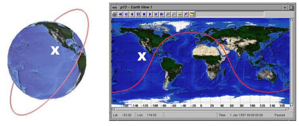
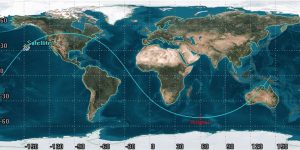
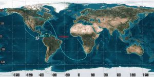
When considering the geometry and physical layout of an orbit, with respect to the earth, we are rarely going to go through the effort of putting together an entire 3D model. A more efficient way to see this relationship is by using what we call a ground track. A ground track is a 2D map of the Earth that shows the path of a spacecraft over Earth’s surface. See Figure 1 as an example.
Even though these can look like nothing more than wavy lines, we can gather a lot from these simple pictures. This includes orbital period, semi-major axis, orbit type, and more.
ROTATING VS NON-ROTATING
Before considering how we will actually define and understand ground tracks, we need to consider a very important assumption. For ground tracks, we are assuming the Earth is rotating because without this assumption we do not learn much about the orbit we are observing. It is simpler to visualize ground tracks on a non-rotating Earth. For a non-rotating earth, since the orbit stays fixed, the ground track will be a perfect sinusoidal wave that loops over the same place over and over again. It will not appear stretched or cut off, but will always be a a sinusoidal wave. This is best shown in the Figure 2 below:
Now, let us consider the Earth rotating. Many aspects of the ground tracks are now going to change. This will add complexity, but we will gain a lot of information about the orbit. The biggest difference one might notice right away for a generic ground track is that the track appears to move westward, such as in Figure 1 shown at the beginning of this chapter:

It is important to note that the satellite has not disappeared into the abyss at this point. Ground tracks typically show only one full orbit. The next orbit would continue from the point where it left off. Note that ground tracks for prograde orbits always have the satellite traveling from left to right. This gap results from the Earth’s rotation, and the closer the period comes to 24 hours the larger this gap gets. This can be seen in Figure 4, where orbit A has a 2.67 hour orbit, B has an 8 hour orbit, C has an 18 hour, and both D and E are geosynchronous and geostationary as the figure eight and single dot indicate, respectively.
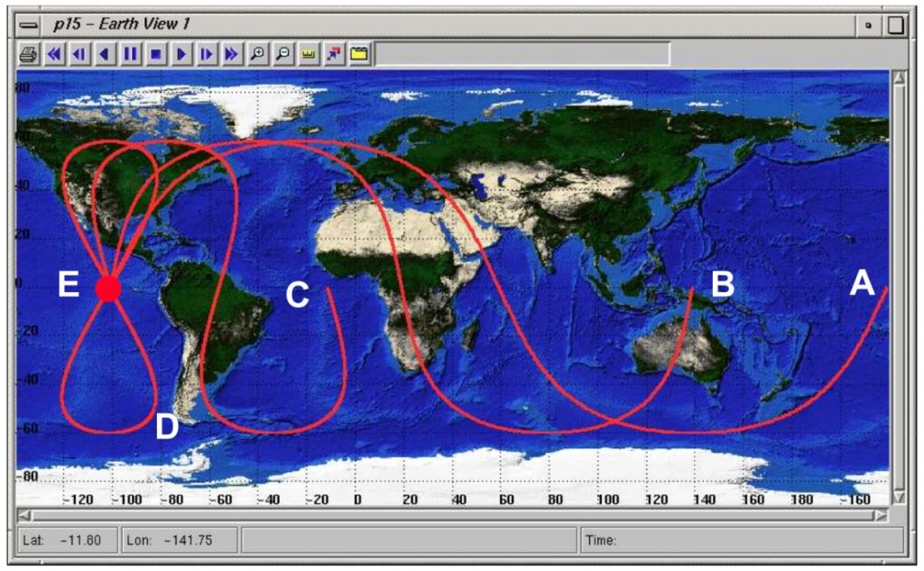
The longer the periods get, the more scrunched the ground tracks are. This is essentially because we are getting closer and closer to the rotation of the Earth, and therefore respective to the surface of the Earth the ground track appears to be stationary in a 24 hour orbit. Another way to think about this is imagine you are standing still on the side of the road and are watching a car drive by. It appears to be going very fast. Now, think about driving next to it in a car going the same speed. The other car will appear to be stationary. It is the same concept here.
From this point forward, we are going to make the assumption that the Earth IS rotating and we will learn to gather information from the ground track.
SEMI-MAJOR AXIS AND TIME OF FLIGHT
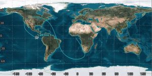
The first variable we are going to define is nodal displacement, [latex]\Delta N[/latex]. This is defined as the longitudinal distance between the ascending nodes. Recall that the ascending node point is where the satellite transitions from the southern hemisphere to the northern hemisphere. Luckily, there is a location on a ground track where it is very easy to spot this– the equator! We are looking for both ascending nodes and finding the longitudinal distance between them (in degrees).
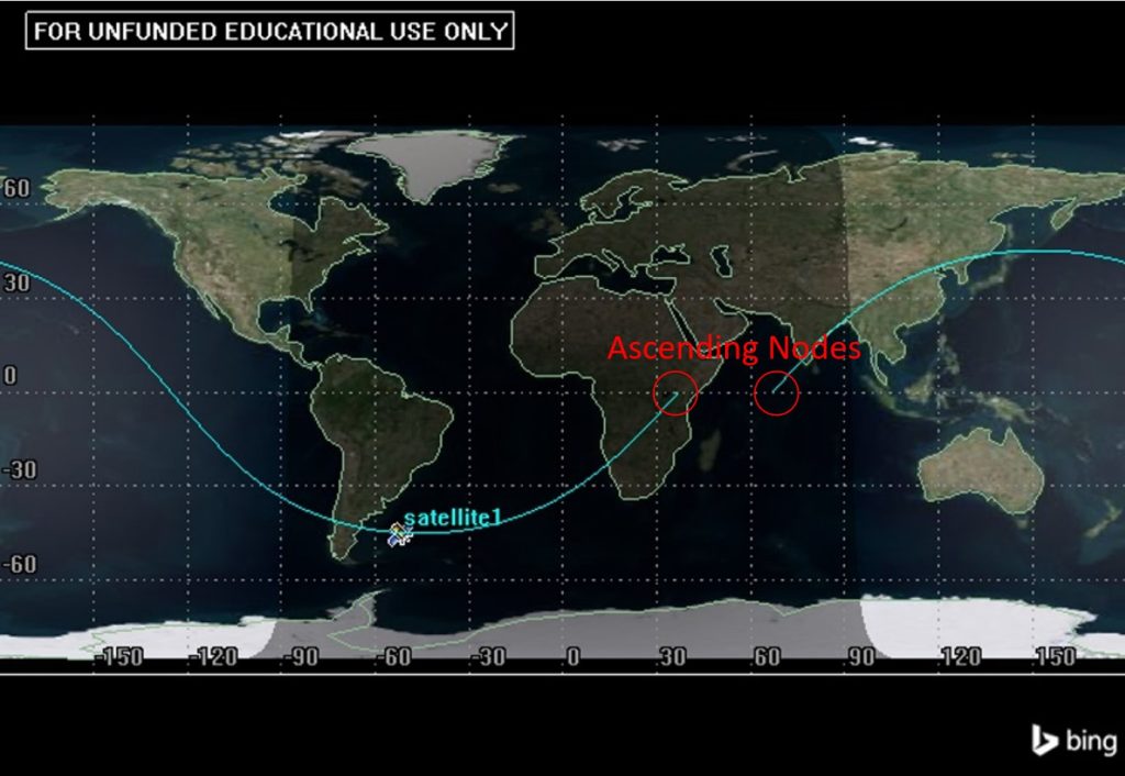
In Figure 5 above, the two ascending nodes are marked with red circles. The gap between them occurs due to the rotation of the Earth as discussed before. On a non-rotating Earth there would only be one ascending node. Determining the gap between these, [latex]\Delta N[/latex], is how we can use this information to determine the semi-major axis of the orbit. There are a few steps to this process and two different methods to determining orbital size. The first is determining the longitudinal distance between the ascending nodes and subtracting it from 360°.
[latex]\large\Delta N = 360° - longitude \;traveled \;between \;ascending \;nodes[/latex]
For example in Figure 6:

Figure 6 shows the longitude between ascending nodes to be 330°. This means we can use this value in the equation to find [latex]\Delta N[/latex].
[latex]\large\Delta N = 360° - 330° = 30°[/latex]
This is one way to find nodal displacement, but there is another way, which can be useful and is less mathematical. This is to measure the literal longitudinal gap between the two ascending nodes, as shown in Figure 7.
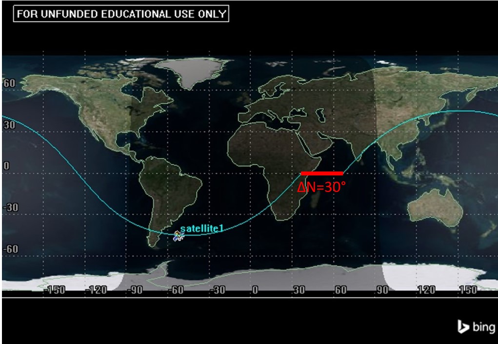
We can see that both of these methods yield the same result of a nodal displacement of 30°.
This is important because this value can be used in the case of direct orbits to find the period of an orbit:
[latex]\large\ P = \frac{\Delta N}{15°/hr}[/latex]
The period can then be used to find the semi-major axis, a, with its relationship as we have defined previously:
[latex]\large\ a=\sqrt[3]{\mu(\frac{P}{2\pi})^2}[/latex]
Inclination
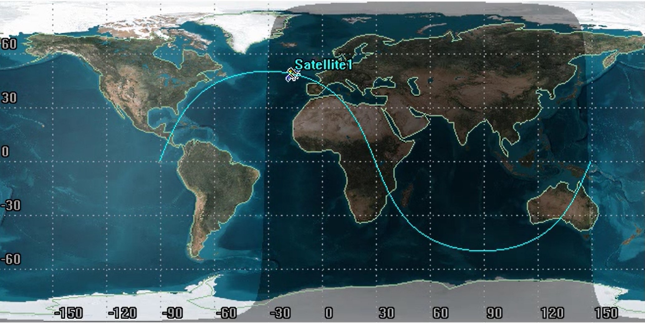
Inclination is also straightforward to read from a ground track. For direct orbits, inclination is the latitudinal distance from the equator to the maximum or minimum of the ground track. For example, see Figure 8:
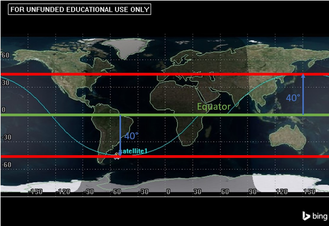
In this example, the inclination is 40°. Note that a satellite in LEO with an inclination of 0° would be a straight line on the equator.
In order to get a better feel for ground tracks, let us consider a few examples.
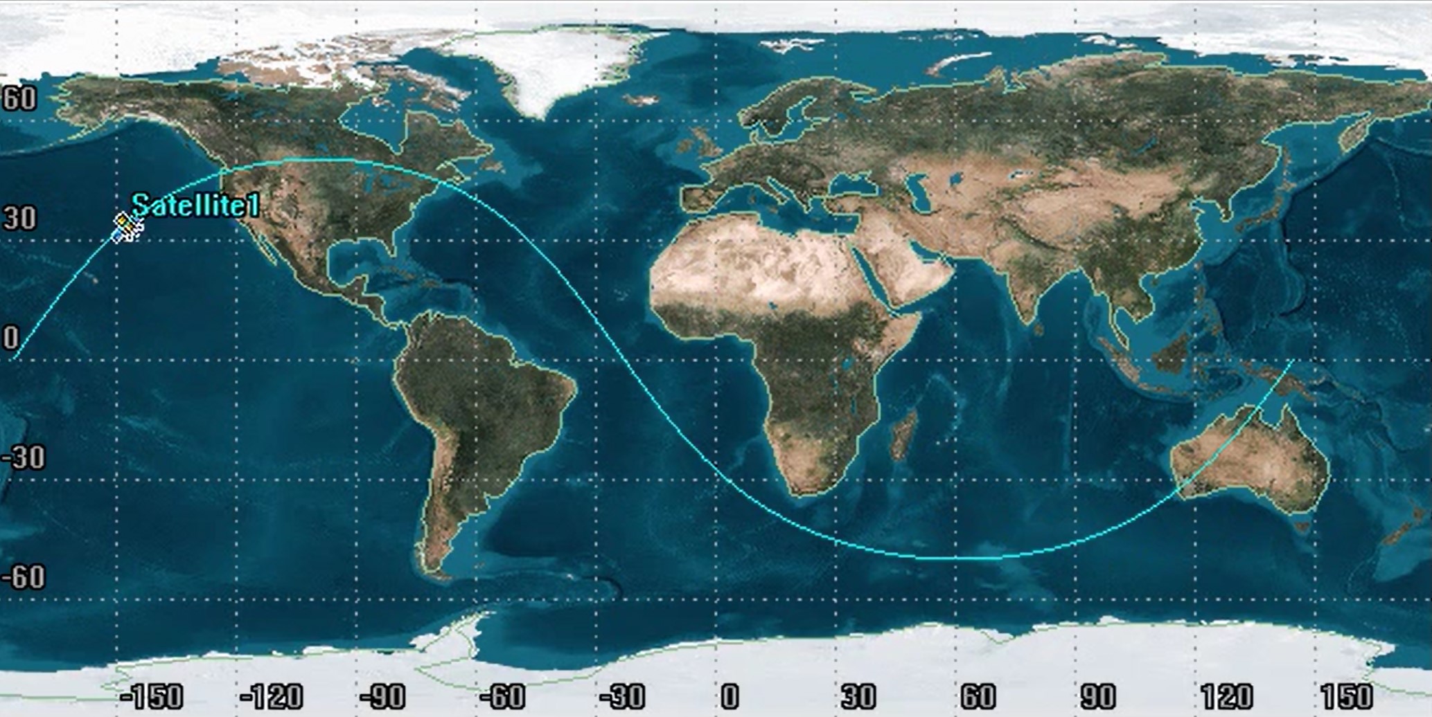
Video 1: Circular LEO 2.67 Hour
The case above has a period of 2.67 hours and is circular. We can tell it is circular because it has line and hinge symmetry, which is talked about later in the chapter. We can read its inclination of ~50° and that it has a [latex]\Delta N[/latex] of a ~40° directly from the ground track. Using the previous equations we can find that the period is approximately 2.67 hours.
Note that you can also determine the alternate orbital element, u, or argument of latitude for this orbit as well. Recall the definition from Chapter 3, an alternate orbital element is the angle between the ascending node vector and the satellite’s position. Since the satellite is nearly at the ascending node, u, would be very small, perhaps about 5°. Likewise, for the first example in the section, u, is approximately 270°. Argument of latitude is only measurable from a ground track for inclinations not equal to 0°.
At this point you might be wondering what an orbit with a 24 hour period looks like. There are two different ways this can look on a ground track. The words geostationary and geosynchronous should be familiar. It just happens that these are our two different cases! A geostationary orbit is the more self-explanatory of the two. As the word “stationary” implies, the orbit looks entirely motionless on a ground track because the satellite is traveling at exactly the same rate as the Earth is rotating.
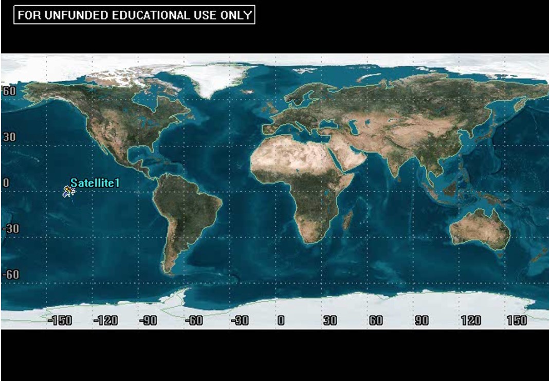
The important part of a geostationary orbit is that it has an inclination of 0. If it does not, it will be a geosynchronous orbit. This will manifest in the form of a figure eight ground track. It will keep its [latex]\Delta N[/latex] of 360° as it has the one ascending node where the figure eight crosses. The inclination can still be read from the latitudinal distance from the equator to the maximum OR the minimum:
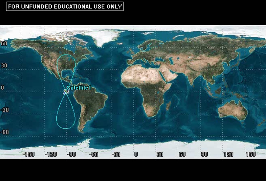
The simulation in Video 2 may help clarify what is happening with a geosynchronous orbit:
Video 2: Circular 24 hours
ECCENTRICITY
So far, these have all been examples of circular orbits with an eccentricity of 0. One thing to understand about ground tracks, with respect to eccentricity, is that the exact eccentricity value cannot be determined if it is not a circular orbit. We can tell if the orbit is circular or elliptical. A circular orbit’s ground track will be more uniform. An elliptical orbit is going to be non-symmetric; i.e. more stretched in some places and more compressed or “scrunched” in others.
We have a way to describe this that is not just “stretched” or “compressed.” To make this determination, we will consider line and hinge symmetry. Take a look at line symmetry. The first step is to take the ground track as a whole and split it in half on the equator where we have a Northern Hemisphere and Southern Hemisphere portion. We are then going to split each of these in half vertically at their peaks (maximum and minimum). If each northern and southern portion is symmetric, then it has line symmetry. This can be viewed best in Figure 11 below:
For hinge symmetry, we again look at the origin. Though, this time, we are going to make the point where the satellite crosses the equator a pivot point. If we can rotate one half of our orbit around that point and it looks the same after being rotated 180° (it will lay on top of the other side perfectly), then it has hinge symmetry. This can be seen in Figure 12 below:
A circular ground track will have both of these features and is both line and hinge symmetric. If it is only symmetric in one type of symmetry and not the other, then it is not circular and therefore its eccentricity is not 0. Here is what the shape of a circular orbit would look like with Figure 13:
Now, let us try a couple of examples!
EXAMPLE 1
Video 3: Circular 8 Hours
Given the ground track seen above, determine eccentricity, period, and altitude.
EXAMPLE 2
Video 4: Circular 18 Hours
Given the ground track seen above, determine eccentricity, period, and altitude.
Attempt this quiz to test your understanding of ground tracks up to this point.
RAAN
Unfortunately, there is no way to determine RAAN from a ground track unless the vernal equinox vector is shown on the ground track. It normally is not, so we cannot determine the angle between the vernal equinox vector and ascending node vector.
ARGUMENT OF PERIGEE
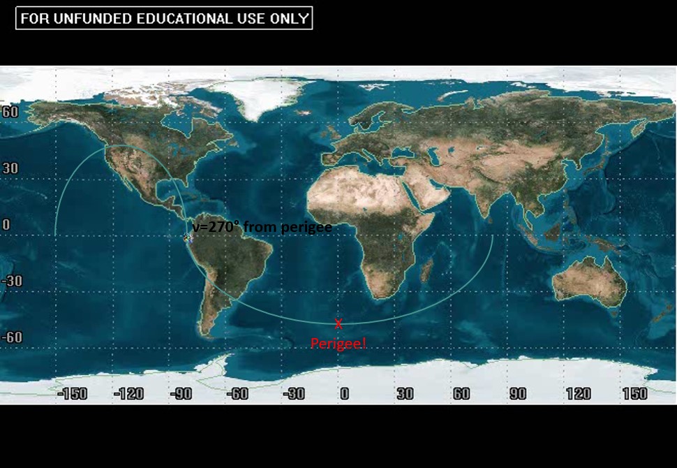
Argument of perigee can also be determined from a ground track. It often takes some practice with visualization of ground tracks in general to get this concept down. Since we are just introducing the idea of ground tracks, let us use visualization to explain how to find this COE from the ground track. Recall, argument of perigee is defined as the angular distance between the ascending node vector and location of perigee. Interpreting the ground track we know where the ascending node is! As a reminder:

We are going to measure the angular distance from the ascending node to perigee from left to right, so we are going to use the “starting” ascending node. This is going to be the node attached to the portion in the Northern Hemisphere when the ascending node is at the end of our ground tracks. We can then use this to determine the angular distance to perigee. At this point, you may be wondering how you determine where perigee is from the ground track.
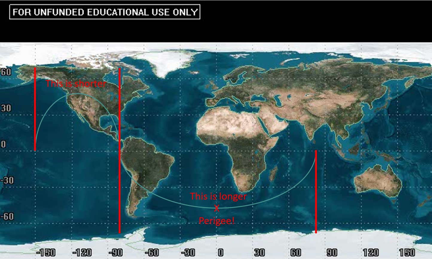
Recall how earlier, with a rotating Earth, the ground track got smaller and smaller the larger the period (and therefore the slower the speed). We are going to use the same reasoning here to find where perigee is. The portions of the ground track where the satellite is moving relatively slow are going to appear “shorter” than the portion of the ground tracks where the satellite is moving relatively fast. Shorter means it is traveling a smaller longitudinal distance to reach a certain point in orbit.
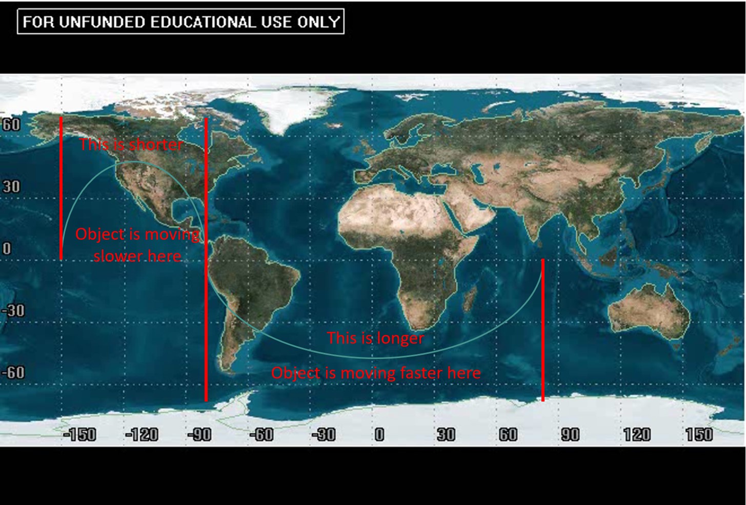
Now, if we think about how an object in orbit is moving at perigee, we will note that it is moving faster than at any other point. We need to determine where it is moving FASTEST. In general, we can use the idea that a satellite is speeding up and slowing down interchangeably to our advantage. In our “long” section, for half of that time the satellite is speeding up and the other half it is slowing down. Therefore, we can determine that perigee is about halfway through the “long” portion of the orbit.
A common error is to read the angle of longitude where perigee occurs and call that the argument of perigee, but that would not be correct. We must refer back to the definition for argument of perigee, which tells us it is the angle between the ascending node and perigee. Again, it might be tempting to read the longitudinal difference between these two points (150°), but that would be incorrect as well.
Recall that we are seeing one full period of an orbit with one ground track. From ascending node to ascending node is 360°, not the measure of the entire map. We can use this to get rough estimates of certain angular distances from the ascending node:
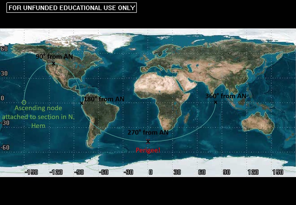
Therefore, in the particular case above, argument of perigee is equal to 270°.
Here are a few videos of simulations showing various arguments of perigees:
Example 1: LEO, [latex]\large\omega = 0°[/latex]
Video 5: Ecc LEO 0
Example 2: MEO, [latex]\large \omega = 90°[/latex]
Video 6: Ecc MEO 90
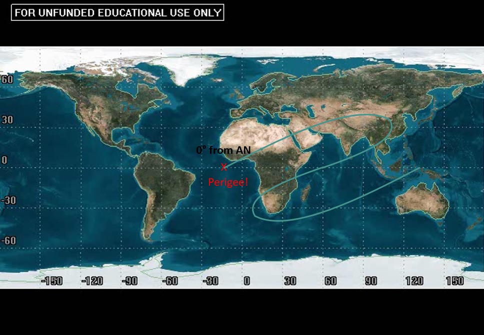
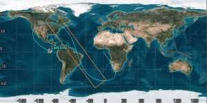
When we talk about “long” and “short” portions of a ground track, what do we do when we come across a track that appears to be moving backwards? In the following image, the object in orbit seems to be doing just that:

Not only does this seem strange, but its “long” portion seems to be the part that is moving backwards. However, this is not where perigee is. Let us first address the appearance of the satellite in the ground track “going backwards”; i.e. moving from right to left. The object itself is not going backwards in its orbit. It just appears to be with respect to the rotating Earth beneath it. This boils down to the Earth moving quicker than the satellite above it, which means the satellite is going VERY slow. Therefore, perigee is definitely not going to be on the stretch in which the satellite appears to be moving backwards. In the example shown above, that eliminates half of the orbit. The other half is going to be “the fast section,” so the middle of that will be its fastest and that is perigee. That portion of the ground track ends up being sliced evenly into two sections, which makes the part where it is cut off perigee. This also happens to be the ascending node, so the distance between the ascending node and perigee leads to an argument of perigee of [latex]\omega = 0°[/latex].
When an orbit is not symmetric in any way, then it might be a little more difficult to read argument of perigee. Specifically, satellites in GEO have very strange looking ground tracks. They come in the dot and figure eight form we discussed with circular GEO orbits, but they can also look like disjointed figure eights, strange teardrop shapes, or even circles! It is very important to note that a circular ground track does not mean a circular obit, but a highly eccentric GEO orbit.
It can be daunting to determine argument of perigee for non-circular GEO orbits, but we can still use the same process to determine argument of perigee.
Video 7: Ecc GEO 180
For Video 7, we have to consider the entire video of its ground track. The first portion is in the Southern Hemisphere and the second is in the Northern Hemisphere. Throughout the entire orbit, the satellite is “going backwards” for half of the orbit, so we can rule that part out for where perigee is. That means perigee will lie halfway through the other half. This lands right on the equator which means it is at ascending or descending node. Watching the video, it hits this point at descending node. The descending node is always 180° from the ascending node. This leaves us with an argument of perigee of [latex]\omega = 180°[/latex].
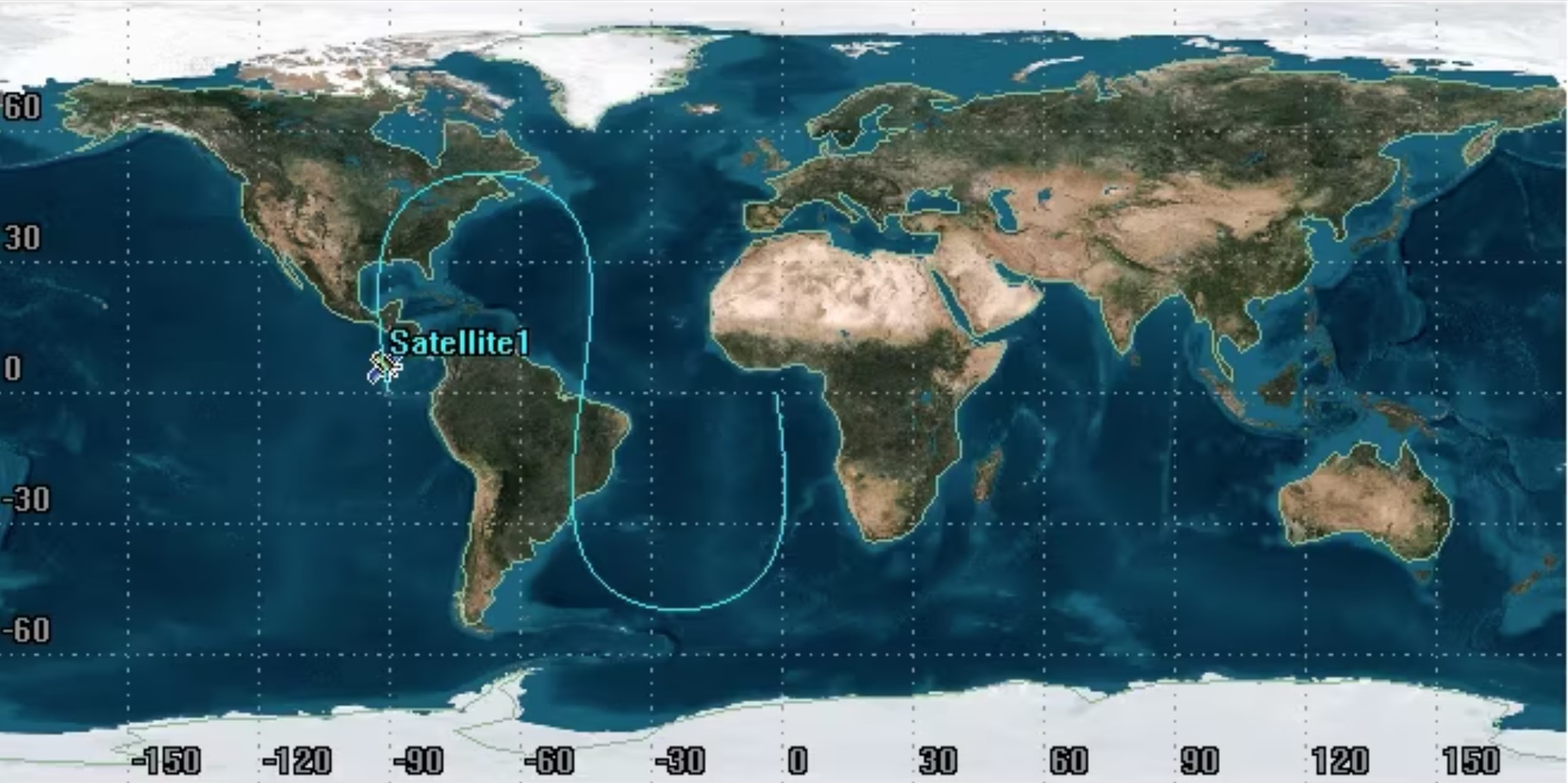
Video 8: Ecc GEO 270
Just like the previous one, this ground track is traveling backwards for half of its orbit (this is a pattern that should be noticed in GEO orbits). The satellite is only traveling forward for the bottom half of the teardrop. So, perigee is at the very bottom of that teardrop shape. If we split the teardrop into four parts– the ascending node, top of the teardrop, descending node, and bottom of the teardrop, being 0°, 90°, 180°, and 270° away from the ascending node respectively– we can define argument of perigee to be [latex]\omega = 270°[/latex]. Again, note that this is measured from the ascending node to the bottom of the teardrop in the direction the satellite is traveling.
TRUE ANOMALY
True anomaly can now be found after perigee is located. Recall that the true anomaly at perigee is by definition 0°. With this information, we can take a similar process to argument of perigee to determine how far away the little satellite icon is from perigee. Using the example from before:

EXAMPLE 3
Video 9: Ecc LEO
Determine argument of perigee, [latex]\omega[/latex].
EXAMPLE 4
Video 10: Ecc MEO 180
Determine the inclination, i, the semi-major axis, a, and the argument of perigee, [latex]\omega[/latex].
In conclusion, ground tracks can be very useful for determining a lot about an orbit. The COEs a, e, and i can be determined for any type of orbit. You can also determine if an orbit is circular or elliptical by considering its line or hinge symmetry. If it is an eccentric orbit, you can further determine argument of perigee, [latex]\omega[/latex], and true anomaly. For a circular orbit, the argument of latitude, u, can also be determined for orbits not at an inclination of 0°.
We have discussed orbits that are determined from the two-body equation of motion. In the next chapter, we will consider which of the assumptions we made when deriving the two-body equation of motion are valid and which are not. In other words, orbits will change over time. We will discuss how to predict those changes, and in some cases, how to make use of these perturbations to design specific types of orbits.
SOLUTIONS TO EXAMPLES:
***EXAMPLE 1 SOLUTION***
Video 3: Circular 8 Hours
Given the ground track seen above, determine eccentricity, period, and altitude.
Solution
Right off the bat, we notice that this ground track appears to have both line and hinge symmetry; therefore, the orbit is circular. This means that:
[latex]\large e=0[/latex]
In this view of the ground track, in order to determine [latex]\Delta N[/latex], let us use the method of taking the longitude traveled between ascending nodes and subtract it from 360°. This is because the entire ground track is visible in one smooth motion and the “gap” is split up. We can observe that the distance traveled between ascending nodes is 240°. Therefore:
[latex]\large \small{\Delta N = 360° - longitude \;traveled \;between \;ascending \;nodes = 360° - 240° = 120°}[/latex]
With the nodal displacement of 120° found, we can determine period:
[latex]\large P = \frac{\Delta N}{15°/hr}=\frac{120°}{15°/hr}=8\:hours[/latex]
This period can then be used to determine semi-major axis with the usual equation:
[latex]\large a = \sqrt[3]{\mu(\frac{P}{2\pi})^2} = \sqrt[3]{398600.5^{km^3}/_{s^2}(\frac{8\:hrs\,*\,\frac{3600\,s}{1\:hr}}{2\pi})^2} = 20,307.4\:km[/latex]
Though the problem did not ask for semi-major axis, it did ask for altitude. We know that altitude is equal to the orbit’s radius minus the radius of the Earth. Luckily, we have already defined this orbit to be circular, so the radius of its orbit is equal to its semi-major axis.
[latex]\large \small{alt = R-R_{Earth}=a_{circular}-R_{Earth} = 20,307.4\;km-6378\;km = 13,929.4\;km}[/latex]
***EXAMPLE 2 SOLUTION***
Video 4: Circular 18 Hours
Given the ground track seen above, determine eccentricity, period, and altitude.
Solution
Just like before, we notice that this ground track appears to have both line and hinge symmetry. This is a little more strange since it doesn’t seem to be a perfect sinusoid as many we have seen before, but it passes both symmetry tests. Therefore, the orbit is circular. Which again gives us an eccentricity of:
[latex]\large e = 0[/latex]
In this view of the ground track, in order to determine [latex]\Delta N[/latex], let us use the method of taking the longitude traveled between ascending nodes and subtract it from 360°. This is because, just like the previous example, the entire ground track is visible in one smooth motion and the “gap” is split up. We can observe that the distance traveled between ascending nodes is 90°. Therefore:
[latex]\large \small{\Delta N = 360° - longitude \;traveled \;between \;ascending \;nodes = 360° - 90° = 270°}[/latex]
With the nodal displacement of 270° found, we can determine period:
[latex]\large P = \frac{\Delta N}{15°/hr} = \frac{270°}{15°/hr} = 18\;hours[/latex]
This period can then be used to determine semi-major axis with the usual equation:
[latex]\large a = \sqrt[3]{\mu(\frac{P}{2\pi})^2} = \sqrt[3]{398600.5^{\,km^3}/_{s^2}(\frac{18\;hr \,*\, \frac{3600\,s}{1hr}}{2\pi})^2} = 34,869.26\;km[/latex]
Though the problem did not ask for semi-major axis, it did ask for altitude. We know that altitude is equal to the orbit’s radius minus the radius of the Earth. Luckily, we have already defined this orbit to be circular, so the radius of its orbit is equal to its semi-major axis.
[latex]\large \small{alt=R-R_{Earth}=a_{circular}-R_{Earth}=24,869.26\;km-6378\;km=28,491.26\;km}[/latex]
***EXAMPLE 3 SOLUTION***
Video 9: Ecc LEO
Determine argument of perigee, [latex]\large \omega[/latex].
Solution
At first glance, it might be tempting to say that this ground track is both line and hinge symmetric. Though, upon closer examination, we can see that it is not.
We can see that the right-hand side is slightly longer than the left-hand side. With this, we know that perigee is halfway between that longer right-hand side:
We can approximate this location to be about ¾ of the way through the orbit. Therefore:
[latex]\large \omega = \frac{3}{4}\,*\,360°=270°[/latex]
***EXAMPLE 4 SOLUTION***
Video 10: Ecc MEO 180
Determine the inclination, i, the semi-major axis, a, and the argument of perigee, [latex]\large \omega[/latex].
Solution
Immediately, we can see that this obit has an inclination of about 50°:
[latex]\large i=50°[/latex]
This ground track does happen to have hinge symmetry but does not have line symmetry, so we know it is not a circular orbit. As always, we are going to start by determining the longitude between ascending nodes. This one might seem a little confusing because the orbit extends past these two points, but we will just be measuring between the two endpoints.

With this:
[latex]\large \small{\Delta N = 360°-\;longitude \;traveled \;between \;ascending \;nodes=360°-90°=270°}[/latex]
With the nodal displacement of 270° found, we can determine period:
[latex]\large P = \frac{\Delta N}{15°/hr} = \frac{270°}{15°/hr}=18\;hours[/latex]
This period can then be used to determine the semi-major axis with the usual equation:
[latex]\large a = \sqrt[3]{\mu(\frac{P}{2\pi})^2} = \sqrt[3]{398600.5^{km^3}/_{s^2}(\frac{18\;hrs\,*\,\frac{3600\,s}{1\,hr}}{2\pi})^2=34,869.26\;km}[/latex]
Now, let us determine the argument of perigee. Part of this orbit is moving “backwards” on the ground track, so we know perigee will not be on those parts. This leaves us with the following section:
The middle part of this section happens to be at the descending node.
We know that the descending node is always 180° from the ascending node, which means:
[latex]\large \omega = 180°[/latex]
REFERENCES
Bate, R. R., Mueller, D. D., & White, J. E. (2015). Fundamentals of astrodynamics. Dover Publications.
Animation of rotating Earth at night.webm. Wikimedia Commons. https://commons.wikimedia.org/wiki/File:Animation_of_Rotating_Earth_at_Night.webm
NASA. (2020, October 5). In depth. NASA. Retrieved March 28, 2023, from In Depth | Hubble Space Telescope – NASA Solar System Exploration
Sellers, J. J., Astore, W. J., Giffen, R. B., & Larson, W. J. Understanding Space An Introduction to Astronautics (3rd ed.). The McGraw-Hill Companies, Inc.
Simple graphic illustration globe showing latitude stock vector (royalty free). Shutterstock. https://www.shutterstock.com/image-vector/simple-graphic-illustration-globe-showing-latitude-13234843
Vallado, D. A., & McClain, W. D. (2013). Fundamentals of Astrodynamics and Applications. Microcosm Press.
Media Attributions
- Figure 6: Longitude Between Ascending Nodes for Satellite 1. © Lynnane Ellis George is licensed under a CC BY-NC-SA (Attribution NonCommercial ShareAlike) license
- Figure 2: Non-Rotating Earth Alongside Sinusoidal Wave Ground Track. is licensed under a CC BY-NC-SA (Attribution NonCommercial ShareAlike) license
- Figure 3: GAP Square Ground Track for Satellite 1. © Lynnane Ellis George is licensed under a CC BY-NC-SA (Attribution NonCommercial ShareAlike) license
- Figure 4: Orbit Gaps (A, B, C, D, and E) Resulting From the Earth’s Rotation. is licensed under a CC BY-NC-SA (Attribution NonCommercial ShareAlike) license
- Figure 5: Two Ascending Nodes Resulting From the Earth’s Rotation. © Lynnane Ellis George is licensed under a CC BY-NC-SA (Attribution NonCommercial ShareAlike) license
- Figure 7: Nodal Displacement Ground Track © Lynnane Ellis George is licensed under a CC BY-NC-SA (Attribution NonCommercial ShareAlike) license
- Figure 8: Inclination Derived From Max and Min of Ground Track for Satellite 1. © Lynnane Ellis George is licensed under a CC BY-NC-SA (Attribution NonCommercial ShareAlike) license
- Figure 9: (Motionless) Ground Track for Geostationary Satellite 1. © Lynnane Ellis George is licensed under a CC BY-NC-SA (Attribution NonCommercial ShareAlike) license
- Figure 10: Ground Track for Geosynchronous Satellite 1. © Lynnane Ellis George is licensed under a CC BY-NC-SA (Attribution NonCommercial ShareAlike) license
- Figure 11: Line Symmetric Process. is licensed under a CC BY-NC-SA (Attribution NonCommercial ShareAlike) license
- Figure 12: Hinge Symmetric Process. is licensed under a CC BY-NC-SA (Attribution NonCommercial ShareAlike) license
- Figure 13: Line and Hinge Symmetric Process. is licensed under a CC BY-NC-SA (Attribution NonCommercial ShareAlike) license
- Figure 14: Satellite Speed Ground Track © Lynnane Ellis George is licensed under a CC BY-NC-SA (Attribution NonCommercial ShareAlike) license
- Figure 15: Argument of Perigee Ground Track © Lynnane Ellis George is licensed under a CC BY-NC-SA (Attribution NonCommercial ShareAlike) license
- Figure 16: Full Argument of Perigee Process GIF © Lynnane Ellis George is licensed under a CC BY-NC-SA (Attribution NonCommercial ShareAlike) license
- Figure 17: Argument of Perigee Ground Track © Lynnane Ellis George is licensed under a CC BY-NC-SA (Attribution NonCommercial ShareAlike) license
- Figure 18: Backwards Section of Ground Track for Satellite 1. © Lynnane Ellis George is licensed under a CC BY-NC-SA (Attribution NonCommercial ShareAlike) license
- Figure 19: Argument of Perigee in a Retrograde Ground Track for Satellite 1. © Lynnane Ellis George is licensed under a CC BY-NC-SA (Attribution NonCommercial ShareAlike) license
- Figure 20: (90 Degrees) True Anomaly Ground Track © Lynnane Ellis George is licensed under a CC BY-NC-SA (Attribution NonCommercial ShareAlike) license
- Figure 21: (270 Degrees) True Anomaly Ground Track © Lynnane Ellis George is licensed under a CC BY-NC-SA (Attribution NonCommercial ShareAlike) license
- Figure 22: Circular Ground Track © Lynnane Ellis George is licensed under a CC BY-NC-SA (Attribution NonCommercial ShareAlike) license
- Figure 23: Line and Hinge Symmetric Process for Satellite 1. © Lynnane Ellis George is licensed under a CC BY-NC-SA (Attribution NonCommercial ShareAlike) license
- Figure 24: Neither Symmetric Process Ground Track © Lynnane Ellis George is licensed under a CC BY-NC-SA (Attribution NonCommercial ShareAlike) license
- Figure 25: Neither Symmetric Process GIF © Lynnane Ellis George is licensed under a CC BY-NC-SA (Attribution NonCommercial ShareAlike) license
- Figure 26: Solved Argument of Perigee for Satellite 1. © Lynnane Ellis George is licensed under a CC BY-NC-SA (Attribution NonCommercial ShareAlike) license
- Figure 27: Solved Inclination for Satellite 1. © Lynnane Ellis George is licensed under a CC BY-NC-SA (Attribution NonCommercial ShareAlike) license
- Figure 28: Longitudinal Distance (90 Degrees) Between Ascending Nodes © Lynnane Ellis George is licensed under a CC BY-NC-SA (Attribution NonCommercial ShareAlike) license
- Figure 29: Potential perigee points © Lynnane Ellis George is licensed under a CC BY-NC-SA (Attribution NonCommercial ShareAlike) license
- Figure 30: Perigee for Elliptical path © Lynnane Ellis George is licensed under a CC BY-NC-SA (Attribution NonCommercial ShareAlike) license
