6 Chapter 6 – Kepler’s Prediction Problem

Let us now return to one of the big pictures of this book. Have you ever looked up at night and seen a bright dot streak across the sky?  That object could be a meteor (shooting star) identified by a trail behind it. However, it could also be a satellite! In the latter case, it will be coming back overhead sometime later. It might be good to know when and where that will be. It would be especially important if you were communicating with the satellite during the time that it is overhead (pass time). You would want to know when and where to point your antenna for the next pass. Or, you might want to know how long it takes a satellite to get to a particular location. These two scenarios make up Kepler’s Prediction Problem.

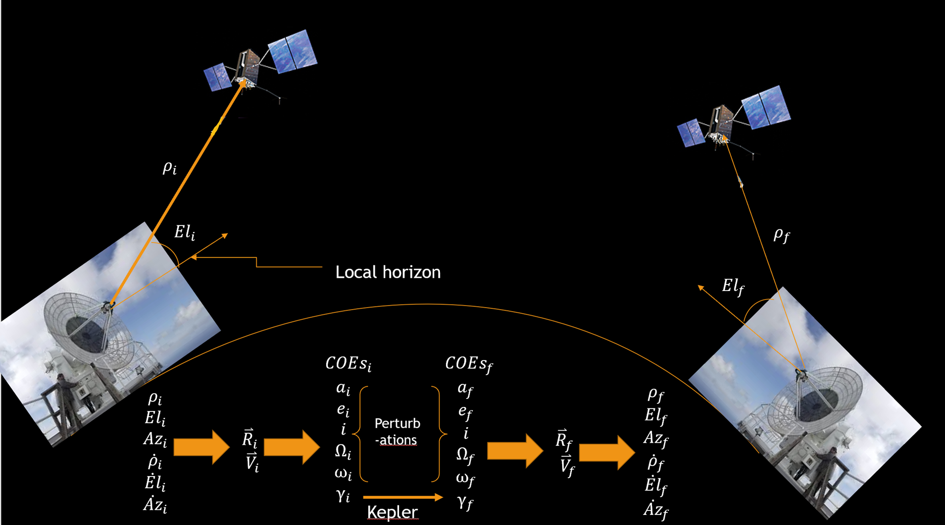
Now we are starting to track data from an initial set to a final set. This requires multiple steps, some of which we have talked about already. We learned about calculating the classical orbital elements, COE’s, using a position and velocity vector. As seen in the image below, one of the next steps is going from an initial set of COE’s to a final set. There are some perturbations that affect most of our COE’s, but what we are focusing on in this chapter is relating initial true anomaly, ν_i, time of flight, TOF, and final true anomaly, ν_f. This problem can be worked two ways.  The first is determining the time it takes for an object in orbit to travel from one position to another (time of flight). The second part is determining where an object will be after a time of flight from a given initial position. Both of these are crucial in astrodynamics and will be discussed in this chapter.

Of course, we have many types of orbits that we have talked about previously. The two we will be focusing on are circular and elliptical orbits. Objects in circular orbits have a constant speed, therefore time of flight and distance traveled can be calculated with ease. In order to make these calculations simpler, let us define a new variable, mean motion, which we will represent with the variable n. This is not to be confused with the ascending node vector, which is dictated with a vector sign, [latex]\vec{n}[/latex]. Mean motion is the average angular speed (in radians per second) of the object in circular or elliptical orbit. For a circular orbit, there are two ways to calculate this value. One way is with the period, P, and the other is with the gravitational parameter of central body, μ, and semi-major axis, a (radius, R, is equivalent to a in circular orbit).

To get from the first way to the second, remember what we define as a period:

So, we can then plug that into the initial equation for mean motion:

Then reducing down, mean motion can be written as the following equation:

This can now be paired with an initial and final argument of latitude, u_i and u_f (note that these are the alternative orbital elements we use for circular orbits instead of true anomaly) to determine time of flight, TOF.

This equation can be rearranged to calculate a future position of final argument of latitude, u_f, if given an initial argument of latitude, u_i and time of flight, TOF.

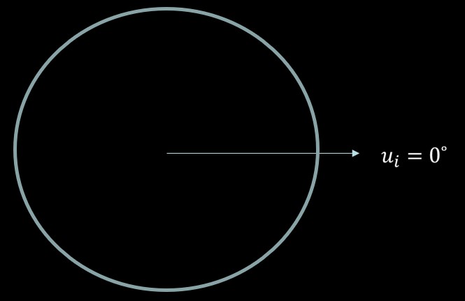
EXAMPLE 1

Given a satellite in a circular orbit with a period of 4 hours has an initial argument of latitude, u_i = 0°, and a time of flight of 6 hours.

Find the final argument of latitude, u_f.

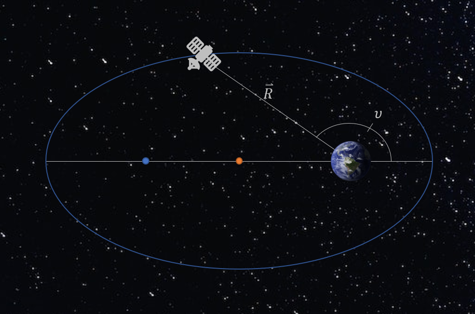
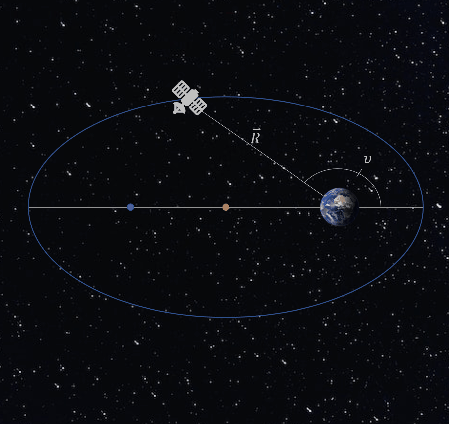
When it comes to elliptical orbits, it is just not as simple as circular orbits due to the speed and, therefore, the true anomaly of the object is not changing uniformly throughout the orbit. Because of this, we need to define a few new variables. Before we do, let us remember how true anomaly is defined so we can properly shift our minds to the new variables. In an elliptical orbit, the Earth lies at one of the foci. The Earth is not at the center of the ellipse, which is one of the reasons why true anomaly does not change uniformly. A true anomaly of 0 radians is defined as the argument of perigee, and a true anomaly of π is defined as the argument of apogee. These can be seen in the image below.

The first of these variables is eccentric anomaly, E. It is defined by first creating a circle (which we call an auxiliary circle) around the ellipse where the radius of the circle is equal to the semi-major axis of the ellipse and centered at the center of the ellipse; i.e. not centered on the Earth. Then, a line is drawn perpendicular to the major axis, going through the point where the object is located and extended to the edge of the circle. Another line is then drawn from the center of the ellipse/circle to the point where the last line drawn and the circle intersect. The angle measured from the major axis to this line is defined as the eccentric anomaly. This process can be observed in the animation below. This creates a direct link between the true anomaly and a way to measure angles that are circular. However, eccentric anomaly still does not change uniformly.

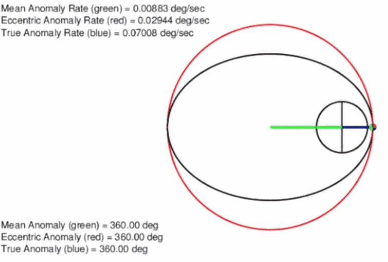
Mean anomaly, M, on the other hand is uniform. It is not as easy to relate these geometrically as they are changing at different rates as opposed to eccentric and true anomaly which travel at a rate equal to each other. One piece of information to note is that the mean anomaly uses the same circle for travel as the eccentric anomaly. It is also important to note that all three anomalies pass both perigee and apogee at the same time. This is why it is called the mean anomaly. It takes the average of the velocities of using eccentric anomaly and keeps the same period. This can be seen better in the following graphic. Calculating this algebraically can be found below in this chapter. Notice that true anomaly, eccentric anomaly, and mean anomaly are all equal to 0 degrees at perigee and π at apogee.

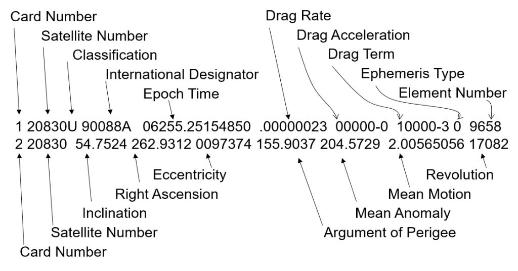
Before continuing with Kepler’s prediction problem, let us talk briefly about Two Line Element Sets, TLE’s. The TLE’s, as the name suggests, are two lines of orbital elements. These can be retrieved from nearly every major object in orbit that is being tracked at any given time. Some of these values in the photo below should be familiar such as eccentricity, e, right ascension (RAAN), Ω, and the newly defined mean anomaly, M. Notice that true anomaly is not given. In real life situations, this is what an engineer would be most likely given in order to determine a satellite’s orbit. Keep these in mind as we will return to them in a later chapter.

TYPE 1

Kepler’s Type 1 prediction problem entails determining the time of flight of an object in an elliptical orbit given its starting and final location, which will most likely be described using some initial and final true anomalies. This is very important in the world of Astrodynamics as there are many situations where a satellite, or some other object, may be in an orbit and we want to know how long it takes for it to travel from one location to another.

In order to accomplish this, both the newly defined eccentric anomaly and the mean anomaly are needed. Using how these anomalies are related to one another and to the initial true anomalies described, it is going to take an “outwards-in” approach starting with the “outward” true anomalies and working our way inwards to the time of flight. This can be seen better described in the figure below.

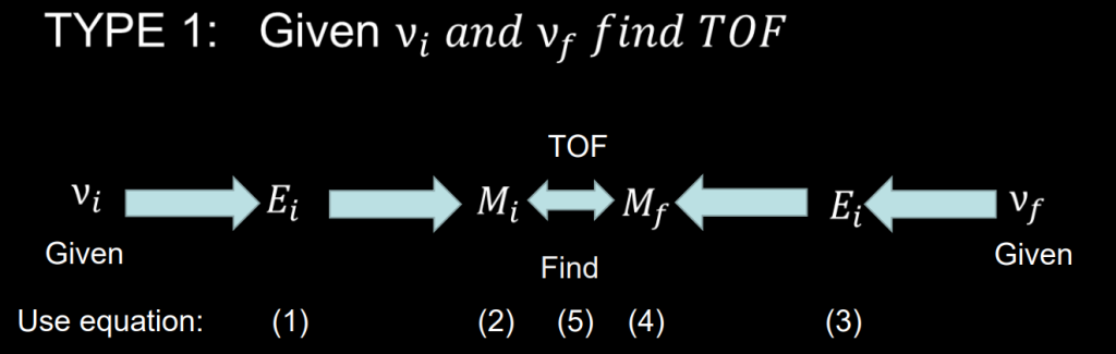
Since this is an outwards-in approach, we can start at either end of the problem and work from there. For the sake of simplicity, we will start at the initial true anomaly, ν_i. We can use this value as well as eccentricity, e, in order to find the initial eccentric anomaly, E_i. This equation can be found below. With that being said, there are issues to look out for in every single step of this process. In this specific process, we have to perform a half plane check. This is just as we did in Chapter 3, when determining the classic orbital elements. It results from the inverse of a cosine producing two different results; the first is in quadrants 1 or 2, the second is in quadrants 3 or 4. In order to account for this, if ν_i>180° then E_i>180°.

Next we will go from initial eccentric anomaly, E_i, to initial mean anomaly, M_i. Again, we use eccentricity, e, in addition to find this value. In this calculation, make sure it is worked in radians. As it can be noticed in the equation below, the value of E_i exists outside of a sinusoidal function, therefore degrees cannot be used.

Going linearly, we will calculate time of flight next; however, we are still missing the final mean anomaly, M_f. So, we need to go to the final true anomaly and work backwards to get where we currently are. First, the final true anomaly, ν_f, and eccentricity, e, would be used to find the final eccentric anomaly, E_f, much like it was done to find the initial eccentric anomaly.  Again, ensure you are performing a half plane check, if ν_f>180° then E_f>180°.

Now we are also going to use the same process to find the final mean anomaly, M_f, as we found the initial. Once again, it is crucial that the equation must be worked out in radians.

Now that we have both mean anomalies, M_i and M_f, we can combine these values with mean motion, n, and finally calculate time of flight! The only piece of information to keep in mind is that it is possible to get a value less than 0. Of course, we cannot have a negative time, so we have to add 2π to the numerator and calculate again. If the value is not less than 0, we have found our time of flight.

For example, if a problem was worked out and a M_i was found to have a value of 3.04 radians, M_f was found to have a value of 1.73 radians, and the mean motion, n, was found to be 5.83×10^-4 rad/s. So if we plug this into the time of flight equation we get:

Now, we see that we have a negative time. So, unless we time traveled, this value is not possible! In order to fix this, all we have to do is add 2π to the numerator and it should return a positive value.

Now that we have a positive value, it is our final time and we can use this as our time of flight.

In summary,

EXAMPLE 2

Given a satellite with the the following COE’s:

a = 26,571 km

e = 0.7

i = 63º

Ω = 180º

ω = 270º

Find the number of hours the satellite spends in the Northern Hemisphere.

Check your understanding with this quick quiz:

TYPE 2

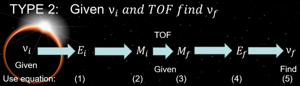
Kepler’s Type 2 prediction problem takes in an initial true anomaly and time of flight in order to determine a final true anomaly.  Instead of outside-in, the Type 2 problem marches directly forward from an initial location to a final location, as seen in the figure below. This is perfect when we want to know where a satellite will be after a certain amount of time.

Finding the initial eccentric and mean anomalies uses the same exact processes and things to look out for as in Type 1. We can use this value as well as eccentricity, e, in order to find the initial eccentric anomaly, E_i. In order to do the half plane check, if ν_i>180° then E_i>180°.

Again, to go from initial eccentric anomaly, E_i, to initial mean anomaly, M_i, use eccentricity, e, in addition to find this value. Be sure to work entirely in radians again.

Determining the final mean anomaly is where things are slightly different than Type 1. First of all, we are going to define a new variable, k. k represents how many times the object in orbit has passed perigee. Sometimes we are given an object that has been in orbit for weeks or months, this means it could have made a full orbit multiple times. To calculate this, we are going to have to do something a bit innovative. We are going to calculate the final mean anomaly, M_f, using the below equation. We will use the below equation to determine the value of k.

If the value is greater than 2π (as you should be working in radians), then it has passed perigee more than once. If it is less than 2π, that is the angle. M_f,0, no matter what, is an equivalent angle. We just want to determine what that angle is between 0 and 2π.

To calculate how many times it has passed perigee, we are going to divide by 2π and floor the answer. This means whatever value you get, you will round DOWN to the nearest whole number. Even if the value you get is 15.977, k will be the value of 15.

Now, let us look back at mean motion, n. For elliptical orbits, we are going to use the equation just dealing with gravitational parameter of central body, μ, and semi-major axis, a, to result in:

We then take all of these pieces and put them together for a final equation for final mean anomaly, M_f, that is a value between 0 and 2π, of:

The final eccentric anomaly, E_f, is also a bit tricky. As you will notice, the below equation has the variable, E_f, both on its own and inside of a sine function. It can be attempted, but there is no simple way to solve this equation algebraically. We call this type of equation a transcendental equation because we cannot solve it analytically, so we will have to look at a numeric approach.

NEWTON’S METHOD

Because we cannot solve for eccentric anomaly analytically, we are going to take a quick departure from Kepler’s Problem and learn a little bit about numerically solving equations. There are many different ways to approach solving equations that cannot be solved with simple algebra. We can solve them using a brute force method, but the method we are mainly going to focus on is Newton’s Method.

The brute force method entails plugging in a value for E_f on the right side of the equation, getting a value, and then using that value to plug back into the right side of the equation again. This is repeated until the result of this gets so similar to the last that it becomes unnoticeable. The first value we will use as E_f is actually M_f. This can be seen in equation form below:

A short example of this can be seen below. 

EXAMPLE 3

Given a satellite with an eccentricity of 0.2 and a final mean anomaly, M_f of 5.07, find the final eccentric anomaly, E_f, using the brute method for 5 iterations.

Though this is an option, it can take much longer than the more efficient Newton’s Method, which is the recommended approach to take.

This method uses the fact that the slope of an equation near a root will point towards said root. As with many numerical methods, an initial guess for the root is needed. This should be somewhat close to the actual root of the function. For an equation y(x), we will call this initial guess x₀. (Note, this can be a bit difficult at times if it is not known where the root is near, but for our purposes, we will always use the final mean anomaly as the initial guess).

We will use a hypothetical function as seen in the graphic below to show how this method works.

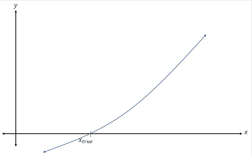
After an initial guess of x₀ is chosen, we follow that point up to y₀ which can also be written as y(x₀). The slope is then taken at that point and followed all the way down past the x-axis. As you can see, the slope is inching towards the real root which has been labeled as xtrue. Let us take a look at that slope. There are multiple ways to describe the slope of a line at a specific point. The first is using the rise over run slope formula:

*Note these are just x₁’s, x₂’s and so forth. These are representing a first point and a second point and do not represent the actual points on the graphic.

The first point is where the slope crosses the x-axis and the second point is the initial guess on the function line (x₀, y(x₀)). Therefore, the rise is from the x-axis to y(x₀) and the run is from where the line crosses the x-axis, which will now be labeled as x1 to the initial guess of x₀. This results in the slope of:

With this, there is another way to write the slope at a given point. This is simply evaluating the derivative of the function at that point. We can write this as:

Both of these ways are completely correct and accurate ways to write the slope of m of the function at the initial guess. Because of this, these two slopes can be set equal to each other resulting in:

With this equation, if both the function is known and the derivative can be taken, everything except x₁ is known. So, let us rearrange this equation to solve for x₁.

We now have x₁ and can repeat this process to find x₂:

As you will notice in the above graphic, this point is even closer to the true solution. We can now write this process in a generic form using n as the current iteration.

This process can potentially be repeated an infinite number of times; however, we can stop iterating whenever we would like. If this is done correctly, every new x calculated should be closer and closer to the last. Once the difference between x_n and x_n+1 is small, we can say that value is the solution. This method is a little more complicated to set up than the brute force method, but it will always converge and arrive at a solution faster.

Back to Type 2

We can now use this method in order to calculate the final eccentric anomaly, E_f. Again, the important thing to look out for when solving is to work in radians. Let us take a look at the formula for E_f again:

We can rearrange this to have everything on one side of the equation to have the formula, f:

E_f is the independent variable, as mean anomaly, M_f, and eccentricity, e, are known at this point. To use Newton’s Method, the derivative of this function must be taken and can be seen below:

Now using Newton’s Method, the iterative formula ends up being:

As stated previously, one of the most difficult parts of Newton’s Method is choosing an initial guess. Luckily, we have an initial guess in M_f:

Let us take a look at a quick example calculating E_f given M_f.

---

EXAMPLE 4

Given a satellite with an eccentricity of 0.2 and a final mean anomaly, M_f, of 5.07, find the final eccentric anomaly, E_f, using Newton’s method for 3 iterations.

---

If more significant figures are needed, then continue iterating.

The final value to calculate for this problem is the final true anomaly. This is what we were after since the beginning of this Type 2 problem. It simply uses the final eccentric anomaly, E_f, and eccentricity, e. Again, you will notice this equation uses an inverse cosine; therefore, we will have to do a half plane check where if E_f>180° then ν_f>180°. Once that is complete, we have finished the problem!

---

EXAMPLE 5

Given a satellite with a time of flight of 1 week and the the following COE’s:

a = 14,596 km

e = 0.197

i = 63º

Ω = 180º

ω = 270º

ν_i = 79.2º

Find ν_f

Use the brute force method to 5 iterations.

---

In summary,

Now, take this quiz to test what you have learned!

The Final Position and Velocity Vectors

Now that we have the updated COE’s, we must find the new position and velocity vectors. Hypothetically, it can be attempted to work this problem backwards from the equations we have for the COES’s, however, that is not reliable. We do have a solid way to calculate these variables given the final COE’s.

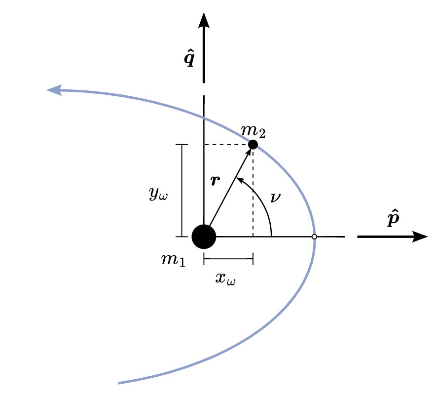
The first step is going to be finding R and V in yet another coordinate frame. The coordinate frame is the PQW (perifocal) frame. This coordinate frame is a frame at a snapshot in time where the P direction is pointing in the x direction, the Q direction is pointing in the y direction, and the W is perpendicular to both of those using the right hand rule.

Firstly, we need to recall the specific angular momentum as well as its magnitude.

This is needed in order to find the value of semi-latus rectum, p.

This can then be used to calculate the magnitude of the final velocity vector. No matter what coordinate frame we are in, the magnitude of R will always be the same. Therefore, we can use it as a bit of a buffer between the PQW and IJK coordinate frames.

This value can then be used to find the values of position and velocity vectors in the perifocal coordinate frames.

Just like when we calculated the initial position and velocity vectors, we used a rotation matrix to translate between the IJK and SEZ coordinate frames, we are going to do the same thing here, though it is going to be a little more complicated. The ultimate rotation matrix is made up of three other rotation matrices. These three are made up of these two base matrices:

ROT1 is used once and uses a negative inclination as its θ and ROT3 is used twice with negative RAAN and argument of perigee being used as θ. The product of these rotation matrices gives the full rotation matrix, which we signify with a tilde (~) over it.

This rotation matrix is then multiplied by the R and V frames in the perifocal coordinate frame. This will help us find the final R and V vectors in the IJK frame.

Next, we need to continue working backwards. Now that we have our position and velocity vectors, we can calculate the final range, azimuth, and elevation. Firstly, the final range in the IJK coordinate frame is found. This uses the same R_site as seen in chapter 4.

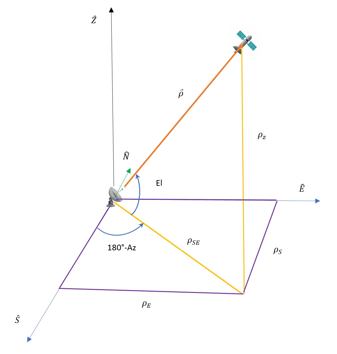
We then use this to move backwards and convert this range into the range in the SEZ coordinate frame. If you need a refresher, here is that coordinate frame:

To get into this coordinate frame, we use the same rotation matrix from Chapter 4. DO NOT use the ROT₁ or ROT₃ spoken about earlier.

With this value, we can find elevation. With elevation, we do not need to worry about plane checks because the value will be between 0º and 90º.

We can calculate azimuth as well. Unlike elevation, azimuth can be a value between 0° and 360°. Because of this, we need to do a plane check.

Despite the fact that these values might be good to have, one might wonder why we need these. Well, it is important to know whether or not we can see the satellite from the site. With the Earth being round, there are some places it cannot be seen. If the range and elevation are in a particular range, we can say it can be seen. These values are:

---

SOLUTIONS TO EXAMPLES:

***EXAMPLE 1 SOLUTION***

Given a satellite in a circular orbit with a period of 4 hours has an initial argument of latitude, u_i = 0°, and a time of flight of 6 hours.

Find the final argument of latitude, u_f.

There are 2 ways to approach this problem: the method of logically thinking it through, and solving it using the equations. Let us start with thinking it through logically.

In a circular orbit, a satellite moves at a uniform speed. With a period of 4 hours, this means the satellite has completed 1.5 orbits in 6 hours (6 hours/4 hours). 1.5 orbits is a total of 540º of travel and a final argument of latitude of u_f = 180º (540º-360º).

Now, let us try solving with the equations.

The first step is solving for mean motion, n. We have multiple equations for this variable, so we have to look at what is given. We are given period, so we will use the equation that uses that:

We can now use that value in the equation we have for final argument of latitude.

Unfortunately, we need a value between 0º and 360º, so all we have to do is subtract 360º until u_f is in that range.

Now, we have our final value, and as it so happens, it matches the value we found when we solved it logically.

***EXAMPLE 2 SOLUTION***

Given a satellite with the the following COE’s:

a = 26,571 km

e = 0.7

i = 63º

Ω = 180º

ω = 270º

Find the number of hours the satellite spends in the Northern Hemisphere.

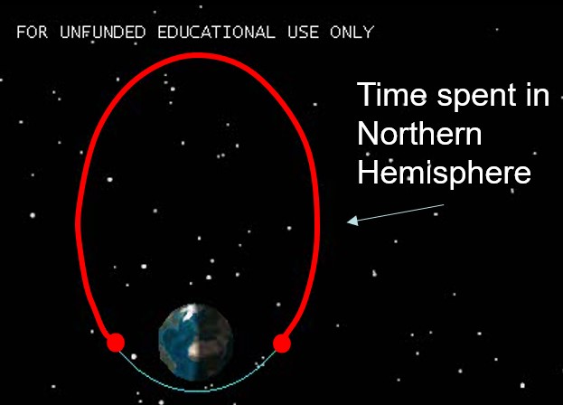
Looking at the following image, or on a whiz wheel, it can be seen that the satellite spends its time from a true anomaly of ν_i = 90º, to a final true anomaly of ν_f = 270º.

Now that we have all the information we need to set up the problem, we can start the algorithm we established for a Kepler type 1 problem. This is starting with finding the initial eccentric anomaly:

With the half plane check, we see that ν_i < 180º(π), so we do not have to amend E_i in any way and we can now find the initial mean anomaly:

Now, we are going to go to step 3 and work inwards from final true anomaly. This starts off with finding final eccentric anomaly:

This time when doing a half plane check, ν_f > 180º(π), therefore we need to amend it so that E_f is also greater than 180º(π).

Now that we have E_f, we can get final mean anomaly:

With this, we have almost every piece of information we need to find time of flight, except mean motion, n. We are going to use the equation that uses semi-major axis, a, as that is a known variable.

Now we have all the pieces to solve for time of flight. Remember to pay attention to units. Using the equation and mean motion in rad/sec, the equation is going to provide an answer in seconds. That answer must be converted to hours.

*Note: We did not use i, Ω, or ω. These are just variables that will be given with any problem that provides COE’s. It is important to descern which of the COE’s you need to use in a specific problem.

***EXAMPLE 3 SOLUTION***

Given a satellite with an eccentricity of 0.2 and a final mean anomaly, M_f of 5.07, find the final eccentric anomaly, E_f using the brute method for 5 iterations.

First we have to get an initial value to use. In our case, we are always going to use M_f as E_f0.

From here, we just take the equation that was initially established for eccentric anomaly and plug in E_f0 on the right hand side of the equation.

This will yield the next E_f value we will use in that place again. We keep doing this until the value converges (or we go however many iterations we are told to, in this case 5):

This leaves us with a final answer of:

***EXAMPLE 4 SOLUTION***

Given a satellite with an eccentricity of 0.2 and a final mean anomaly, M_f, of 5.07, find the final eccentric anomaly, E_f using Newton’s method for 3 iterations.

***EXAMPLE 5 SOLUTION***

Given a satellite with a time of flight of 1 week and the the following COE’s:

a = 14,596 km

e = 0.197

i = 63º

Ω = 180º

ω = 270º

ν_i = 79.2º = 1.3823 rad

Find ν_f.

Use the brute force method to 5 iterations.

The start of this process is quite simple. We just use the equation to solve for the initial eccentric anomaly:

Since this value is less than π, the half plane check is passed and we need to do nothing further but calculate the initial mean anomaly:

To calculate the final mean anomaly, we are going to need mean motion, n, and time of flight, TOF, in seconds:

With this, we can calculate a final mean anomaly:

The issue remains that we need this value between 0 and 2π, which we are currently well above. To account for this, we need to figure out how many times the satellite has passed perigee with the k value. Do not forget to floor the value you get or you could run around in circles:

We can now use this k value in the updated equation to find the equivalent angle for final mean anomaly:

To start finding the final eccentric anomaly using brute force, we need an initial value. As always, we are going to use the final mean anomaly, M_f:

We can now iterate through using the brute force method for 5 iterations using each answer on the right hand side as the variable on the left hand side:

The last step to calculate final true anomaly with the equation:

Doing a half plane check, E_f is greater than π, therefore ν_f must also be greater than π:

This leaves a final result of:

References

Bate, R. R., Mueller, D. D., &amp; White, J. E. (2015). Fundamentals of astrodynamics. Dover Publications.

Animation of rotating Earth at night.webm. Wikimedia Commons. https://commons.wikimedia.org/wiki/File:Animation_of_Rotating_Earth_at_Night.webm

“Perifocal Frame.” Perifocal Frame – Orbital Mechanics & Astrodynamics, https://orbital-mechanics.space/classical-orbital-elements/perifocal-frame.html.

Sellers, J. J., Astore, W. J., Giffen, R. B., &amp; Larson, W. J. Understanding Space An Introduction to Astronautics (3rd ed.). The McGraw-Hill Companies, Inc.

Simple graphic illustration globe showing latitude stock vector (royalty free). Shutterstock. https://www.shutterstock.com/image-vector/simple-graphic-illustration-globe-showing-latitude-13234843

Vallado, D. A., & McClain, W. D. (2013). Fundamentals of Astrodynamics and Applications. Microcosm Press.