SATELLITE CONTROL NETWORKS

Now that we know how to describe a satellite in orbit in terms of its position and velocity vectors, as well as its orbital elements, we will next consider how a satellite’s ground tracking station tracks a satellite. In other words, through observations from a tracking station on the ground, we can tell exactly where a satellite is. Later, we may want to predict where it will be at some point in the future so that we can acquire data or transmit commands to it. We will refer to these ground stations as part of the spacecraft tracking and communication network.

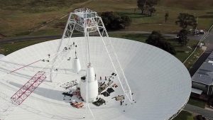
NASA has its own Space Network (SN) to track and communicate with satellites in orbit. The SN empowers missions with reliable and secure relay communications and tracking services. The SN’s global coverage enables near-continuous, bidirectional communications. The SN’s architecture is comprised of two segments. The space segment consists of a constellation of Tracking and Data Relay Satellites (TDRS) in geosynchronous orbit, introduced in the introductory chapter of this textbook (NASA).  A series of ground-based antennas make up the network’s ground segment. A 70-meter-wide (230-foot-wide) radio antenna, Deep Space Station, in Canberra, Australia is shown in Figure 1 below.

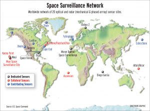
The Air Force also has a Satellite Control Network, which consists of satellite control centers, tracking stations, and test facilities located around the world. Satellite Operations Centers, SOCs, are located at Schriever Air Force Base near Colorado Springs, Colorado and various other locations around the continental United States. The SOCs are manned around the clock and are responsible for the command and control of their assigned satellite systems and are also linked to remote tracking stations, RTSs, around the world. The RTSs provide the link between the satellites and the SOCs. The worldwide locations of the AFSCN are shown below in Figure 2 (Space News).

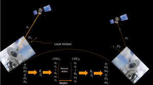
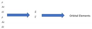
In this chapter, we will concentrate on the observation data we might obtain from a typical ground station and learn how to convert those measurements into position and velocity vectors for the satellite. This initial observation data, or a satellite’s tracking data, is called an ephemeris. Later in this book, we will discover how to predict where a satellite will be in the future using an initial ephemeris and Kepler’s Predication problem. Given future orbital elements, we will determine how to obtain observation data for a ground station to communicate with the satellite at a specified time. This concept is pictured below in Figure 3:

We will first use a series of location parameters from the tracking station and their rates, as measured from a coordinate frame centered at the tracking station.  These parameters are given as:

[latex]\large \rho[/latex]:  Range = distance from tracking station to satellite, usually in km.

Az:  Azimuth = the angle measured from North, clockwise (as viewed from above) to the location on the Earth beneath the object of interest.  It can take values 0 [latex]\leq[/latex]Az [latex]\leq[/latex] 360 degrees

El:  Elevation = the angle measured from the local horizon (tangent to the earth’s surface) to the radar line of site.   Although it can take angles from -90 degrees [latex]\leq[/latex] El [latex]\leq[/latex] 90 degrees, only those satellites with elevations greater than about 20 degrees can be “seen” from a ground station.

[latex]\large \dot{\rho}[/latex]:  Range Rate = the rate at which the satellite is moving relative to to the ground station.  It can have positive or negative values and is usually measured in km/s.

[latex]\large \dot{Az}[/latex]: Rate of Change of Azimuth = the rate at which the satellite is changing azimuth.  It can have positive or negative values and is usually measured in degrees/second or radians/second.

[latex]\large \dot{El}[/latex]:  Rate of Change of Elevation = the rate at which the satellite is changing elevation.  It can have positive or negative values as is usually measured in degrees/ second or radians/second.

But notice where we are measuring them from. We are measuring them from the tracking site; therefore, we must introduce a new coordinate frame: SEZ.

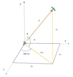
THE SEZ, SOUTH-EAST-ZENITH, COORDINATE FRAME

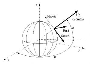
The SEZ coordinate frame, sometimes called the Topocentric Horizon Coordinate System, will be used to define the satellite’s initial location.  It is shown in Figure 4 below.

Now, we will consider a side view of the satellite in orbit. (Note: Figure 5 is not to scale):

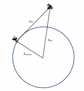
So, we see that Equation (1):

(1)

[latex]\large \vec{R} = \vec{R}_{\text{site}} + \vec{\rho}[/latex]

But is it really that easy? Not exactly, but it’s not that hard if you keep in mind Figure 1 and the coordinate frames attached to each vector. First, let us consider those coordinate frames, indicated by the subscripts in the following Equation (2):

(2)

[latex]\large \vec{R}_{IJK} = \vec{R}_{\text{site}IJK} + \vec{\rho}_{SEZ}[/latex]

Can vectors in different coordinate frames be added? No more than units of feet and meters can directly be added together. There must be a conversion factor between the two references. The same holds true for vectors – there must be a conversion factor between the two reference frames. In vector analysis, this is called a coordinate transformation.

TRANSFORMATION BETWEEN SEZ AND IJK COORDINATE FRAMES

Why is a coordinate transformation needed in this instance? Well, the radar site observations ([latex]\rho[/latex], Az, and El) are measured from the ground site. It is important to know that ground site moves with the Earth.  It is not an inertial coordinate frame, while the IJK frame is inertial. The relationship between the IJK and SEZ frames are shown in Figure 6 below.

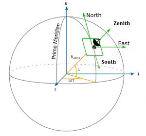
Where:

R_earth = Radius of the Earth, the distance from the center of the Earth to the ground station site (at 0 altitude), km

LST = Local Sidereal Time (degrees), time measured from the [latex]\large \hat{I}[/latex] vector, or principle axis, to current location on the Earth.  More about sidereal time will be discussed in Chapter 6, but we will use it for now because it is an inertial reference frame.

L = latitude (degrees)

In order to proceed further, we will need to find expressions for the quantities x and z in Figure 7, as can be seen from the orange highlighted right triangle.

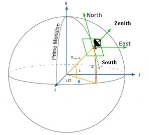
The equations for x and z hence become Equations (3) and (4):

(3)

[latex]\large x = R_{\text{earth}} \cos L[/latex]

and

(4)

[latex]\large z = R_{\text{earth}} \sin L[/latex]

Now also considering the projection on the IJ plane in Equation (5):

(5)

[latex]\large \vec{R}_{\text{site}} = x \cos(\text{LST}) \hat{i} + x \sin(\text{LST}) \hat{j} + z \hat{k}[/latex]

Combining the last two equations yields Equation (6):

(6)

[latex]\large \vec{R}_{\text{site}} = R_{\text{earth}}\cos L \cos(\text{LST}) \hat{i} + R_{\text{earth}}\cos L \sin(\text{LST}) \hat{j} + R_{\text{earth}}\sin L \hat{k}[/latex]

This equation (6) would be a pretty good approximation for [latex]\large \vec{R}_{\text{site}}[/latex] except for two facts.

1. The earth is not spherically symmetrical
2. The site may not be at sea level.

For example, Schriever Space Force Base is at an altitude of 1894 m (6214 ft) and Air Force’s Maui Ground Tracking Station is at a whopping 3058 meters (10032 ft) (Pike, Schriever).

We will start by addressing the first point: how we can account for the Earth’s oblateness.

 EARTH’S OBLATENESS

We could simply use a spherical Earth model, but in order to be more accurate we will need to consider a non-spherical Earth. The first Vanguard satellite revealed that Earth is slightly pear-shaped—an effect we will explore further later. However, a reference ellipsoid is a good approximation to “mean sea level” (Bate)

The Earth can be modeled fairly accurately as a type of ellipsoid, or a stretched sphere. In Figure 8 below, two types of ellipsoids are shown (Math).

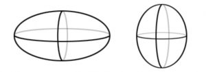
The ellipsoid on the left is an oblate spheroid; the one on the right is a prolate spheroid. The Earth takes the shape of an oblate spheroid due to the rotation of the Earth, which causes the Earth to swell more at the equator than at the poles. When the Earth rotates, there is a strong outward force on Earth matter that is near the equator. This means the radius of the Earth at the equator is approximately 6,378.145 km, while the distance from the center of the Earth to the poles is slightly less, at about 6,356.785 km.  The Earth’s eccentricity is 0.08182.  This results in the geometry in Figure 9 below.

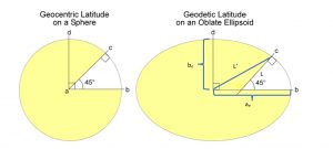
Where:

L = Geodetic latitude, measured from the perpendicular to the Earth’s surface to the point where the line crossed the equatorial plane.

L’ = Geocentric latitude

What we are accustomed to using on Earth is the Geodetic latitude, L.

Consider what would happen in real life if a person dropped a plumb bob and it pointed toward the center of the Earth (Figures 10 and 11)!

In this case, using Geodetic Latitude, more accurate expressions are obtained for x and z in Equations (7) and (8).

(7)

[latex]\large x = \left[ \frac{a_e}{\sqrt{1 - e^2 \sin^2 L}} + H \right] \cos L[/latex]

and

(8)

[latex]\large z = \left[ \frac{a_e (1 - e^2)}{\sqrt{1 - e^2 \sin^2 L}} + H \right] \sin L[/latex]

where

a_e = R_earth = 6378.137 km

e = e_earth = 0.08182

____________________________________________________

Example 1

Given a radar tracking site at:

L = Latitude = 42 degrees

H = altitude above sea level = 77 meters

LST = local sidereal time = 256 degrees

Find

[latex]\large \vec{R}_{\text{site}}[/latex]

___________________________________________________

POSITION VECTOR

But we must remember that [latex]\large \vec{\rho}[/latex] is referenced to the SEZ coordinate frame.

In other words, Equation (9):

(9)

[latex]\large (\vec{R})_{IJK} = (\vec{R}_{\text{site}})_{IJK} + (\vec{\rho})_{SEZ}[/latex]

The above equation will not work because, in order to add vectors, all must be referenced to the same coordinate frame!

Now considering Figure 12’s yellow triangle in Equations (10) and (11):

(10)

[latex]\large \rho_{SE} = \rho \cos(\text{El})[/latex]

and

(11)

[latex]\large \rho_{Z} = \rho \cos(\text{El})[/latex]

Then, considering the purple box in Equations (12), (13), (14), (15), and (16):

(12)

[latex]\large \vec{\rho}_S = \rho_{SE} \cos(180 - \text{Az}) \hat{S}[/latex]

so

(13)

[latex]\large \vec{\rho}_S = -\rho_{SE} \cos(\text{Az}) \hat{S}[/latex]

and

(14)

[latex]\large \vec{\rho}_E = \rho_{SE} \sin(180 - \text{Az}) \hat{E}[/latex]

so

(15)

[latex]\vec{\rho}_E = \rho_{SE} \sin(\text{Az}) \hat{E}[/latex]

and

(16)

[latex]\large \vec{\rho}_Z = \rho \sin(\text{El}) \hat{Z}[/latex]

Now we end up with a final set of Equations (17), (18), and (19):

(17)

[latex]\large \rho_S = -\rho \cos(\text{El}) \cos(\text{Az})[/latex]

and

(18)

[latex]\large \rho_E = \rho \cos(\text{El}) \sin(\text{Az})[/latex]

and

(19)

[latex]\large \rho_Z = \rho \sin(\text{El})[/latex]

But it still does not work! We will need a coordinate transformation between the IJK and SEZ coordinate frames in Equation (20).

(20)

[latex]\large \vec{\rho}_{IJK} = \begin{bmatrix} \sin L \cos \text{LST} & - \sin \text{LST} & \cos L\cos\text{LST} \\ \sin L \sin\text{LST} & \cos\text{LST} & \cos L \sin \text{LST}  \\ -\cos L & 0 & \sin L \end{bmatrix} \vec{\rho}_{SEZ}[/latex]

Where we will define in Equation (21):

(21)

[latex]\large \vec{\rho}_{IJK} = \text{ROT} \vec{\rho}_{SEZ}[/latex]

See Bate for more information.

Now we can add the vectors since they are all referenced to the IJK coordinate frame in Equation (22).

(22)

[latex]\large \vec{R} = \vec{R}_{\text{site}} + \vec{\rho}[/latex]

________________________________________________

Example 2

Given satellite parameters as spotted by the radar tracking station in Example

[latex]\large {\rho}[/latex] = 7000 km

Az = 40 degrees

El = 45 degrees

Find the position of the satellite, [latex]\large \vec{R}[/latex] , in the IJK coordinate frame.

________________________________________________

VELOCITY VECTOR

Now all that is needed is the velocity vector, [latex]\large \vec{V}[/latex] , to find all of the satellite’s COEs.  Recall Equation (23),

(23)

[latex]\large \vec{R} = \vec{R}_{\text{site}} + \vec{\rho}[/latex]

So to find the velocity vector, [latex]\large \vec{V}[/latex] , it will be Equations (24) and (25):

(24)

[latex]\large \vec{V} = \frac{d}{dt} \vec{R}_{IJK}[/latex]

and

(25)

[latex]\large \vec{V} = \frac{d}{dt} (\vec{R}_{\text{site}} + \vec{\rho})[/latex]

Thus Equation (26) will be:

(26)

[latex]\large \vec{V} = \frac{d}{dt} \vec{R}_{\text{site}} + \frac{d}{dt} \vec{\rho}[/latex]

and since the range site is not moving around (typically!) on the surface of the Earth, then Equation (27):

(27)

[latex]\large \vec{V} = \frac{d}{dt} \vec{R}_{\text{site}} = 0[/latex]

So Equation (28),

(28)

[latex]\large \vec{V} = \frac{d}{dt} \vec{\rho}[/latex]

However, since [latex]\large \vec{\rho}[/latex] is attached to the Earth’s surface, which is rotating, transport theorem from dynamics must be used. Recall, to take the derivative of a vector [latex]\large \vec{A}[/latex] in a moving frame in Equation (29):

(29)

[latex]\large \dot{\vec{A}} = \dot{\vec{R}} + \vec{\omega} \times \vec{A}[/latex]

Where the variables for Equations (29) shall represent the following:

[latex]\large \dot{\vec{A}}[/latex] = Derivative of vector A relative to the inertial frame, I

[latex]\large \dot{\vec{R}}[/latex] = Derivative of vector A relative to the moving frame, R

[latex]\large {\omega}[/latex] = Angular velocity of frame R relative to the intertial frame, I

[latex]\large \vec{V}_{IJK} = \frac{d}{dt} \vec{R}_{IJK} = \dot{\vec{\rho}}_{IJK} + \vec{\omega} \times \vec{R}_{IJK}[/latex]

Notice Equation (34):

(34)

[latex]\large \dot{\vec{\rho}}_{IJK} = \text{ROT} \dot{\vec{\rho}}_{SEZ}[/latex]

Where [latex]\large \dot{\vec{\rho}}_{SEZ}[/latex] is determined from taking the derivative of [latex]\dot{\vec{\rho}}_{SEZ}[/latex] and yields Equation 35:

(35)

[latex]\large \dot{\vec{\rho}}_{SEZ} = \begin{bmatrix} -\dot{\rho} \cos(El) \cos(Az) + \rho \dot{El} \sin(El) \cos(Az) + \rho \dot{Az} \cos(El) \sin(Az) \\ \dot{\rho} \cos(El) \sin(Az) - \rho \dot{El} \sin(El) \sin(Az) + \rho \dot{Az} \cos(El) \cos(Az) \\ \dot{\rho} \sin(El) + \rho \dot{El} \cos(El) \end{bmatrix}[/latex]

Where the angular velocity [latex]\large \vec{\omega}[/latex] of the SEZ frame relative to the inertial, IJK frame, which gives Equation 36:

(36)

[latex]\large \vec{\omega} = \begin{bmatrix} 0 \\ 0 \\ 15.041^\circ / \text{hr} \end{bmatrix} \times \begin{bmatrix} \frac{0}{\text{hr}} \\ \frac{0}{3600 \text{ secs}} \\ \frac{\pi}{180^\circ} \end{bmatrix} = \begin{bmatrix} 0 \\ 0 \\ 7.292082578 \times 10^{-5} \text{ rad/s} \end{bmatrix}[/latex]

This type of Preliminary Orbit Determination, as shown in Figure 13, is called COMFIX (complete fix).

Given:                                                                                     Find:

OTHER TYPES OF ORBIT DETERMINATION

OTHER TYPES OF ORBIT DETERMINATION

Comfix is one type of an orbit determination problem and requires the range site data. Alternative methods of determining a satellite’s orbit are possible if other parameters are available. Below are a few other methods and are briefly mentioned and described. For more information, see the references.

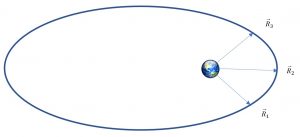
Gibbsian Method

The Gibbsian orbit determination method determines an orbit from three position vectors. It is attributed to Joshua Gibbs (1839 – 1903), an engineer who was believed to be the first American contributor to celestial mechanics. Gibbs is more well-known for his contributions to thermodynamics, but his work in orbit determination is the basis for many current orbit determination methods.

When three position vectors, [latex]\vec{R}[/latex], are known over a relatively long time, you can determine the satellite’s orbit. As shown in Figures 14 and 15 below:

Given:                                       Find:

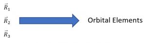
Where (Vallado) in Equation (37):

(37)

[latex]\large \vec{R}_1 \text{ to } \vec{R}_3 > 5^\circ[/latex]

Note that you do not need to know anything about the rate of change of the vectors.

Herrick-Gibbs Method

The Herrick-Gibbs orbit determination method also determines an orbit from three position vectors but requires that they be gathered over a short amount of time. It is not as robust as the Gibbs method, but three closely related space positions may be the only information available due to ground radar site limitations. It is attributed to Sam Herrick (1911 – 1974), who corresponded regularly with Robert Goddard. Herrick said that Goddard’s encouragement led him to anticipate the basic problems of space navigation (Samuel Herrick).

When three position vectors, [latex]\vec{R}[/latex], are known over a relatively short time, you can determine the satellite’s orbit.  As shown in the Figures 16 and 17 below:

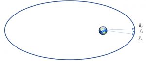
Given:                                       Find:

Where (Vallado) in Equation (38):

(38)

[latex]\large \vec{R}_1 \text{ to } \vec{R}_3 < 1^\circ[/latex]

Note that you do not need to know anything about the rate of change of the vectors.

Gauss-Lambert-Euler

The Gauss-Lambert-Euler orbit determination method determines an orbit from two position vectors and a time of flight between the two. As Lambert first formed the solution, it is better known as Lambert’s problem. It was first posed in the 18th century by Johann Lambert (1728 – 1777), who is known for proving that [latex]\text { П }[/latex] is an irrational number.  The problem was formally solved with mathematical proof by Joseph Lagrange.

When two position vectors, [latex]\large \vec{R}[/latex], are known and a time of flight is known between the two, the orbit between the two positions may be found. This can be seen in Figures 18 and 19 below:

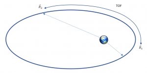
                                                                                     Given:                                       Find:

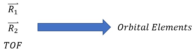
Where Equation (39):

(39)

[latex]\large \vec{R}_1 \text{ to } \vec{R}_2 > 60^\circ[/latex]

Lambert’s problem is often used for interplanetary trajectories.

Complete this quick quiz in order to see how well you understand the concepts from this section.

In the next section, Local Sidereal Time (LST) will be introduced as well as ground tracks.

SOLUTIONS TO EXAMPLES:

***Example 1 Solution***

Given a radar tracking site at:

L = Latitude = 42 degrees

H = altitude above sea level = 77 meters

LST = local sidereal time = 256 degrees

Find

[latex]\large \vec{R}_{\text{site}}[/latex]

Solutions in:

[latex]\large \vec{R}_{\text{site}} = x \cos(\text{LST}) \hat{i} + x \sin(\text{LST}) \hat{j} + z \hat{k}[/latex]

Where:

[latex]\large x = \left[ \frac{a_e}{\sqrt{1 - e^2 \sin^2 L}} + H \right] \cos L[/latex]

[latex]\large x = \left[ \frac{6378.137}{\sqrt{1 - 0.08182^2 \sin^2 42}} + 0.077 \right] \cos 42[/latex]

x = 4747.06 km

and

[latex]\large z = \left[ \frac{a_e(1 - e^2)}{\sqrt{1 - e^2 \sin^2 L}} + H \right] \sin L[/latex]

[latex]\large z = \left[ \frac{6378.137(1 - 0.08182^2)}{\sqrt{1 - 0.08182^2 \sin^2 42}} + 0.077 \right] \sin 42[/latex]

z = 4245.65 km

[latex]\large \vec{R}_{\text{site}} = x \cos(\text{LST}) \hat{i} + x \sin(\text{LST}) \hat{j} + z \hat{k}[/latex]

[latex]\large \vec{R}_{\text{site}} = 4747.06 \cos 25.6 \hat{i} + 4747.06 \sin 25.6 \hat{j} + 4239.15 \hat{k}[/latex]

so

[latex]\large \vec{R}_{\text{site}} = -1148.42 \hat{i} - 4606.05 \hat{j} + 4245.65 \hat{k}[/latex]

***Example 2 Solution***

Given satellite parameters as spotted by the radar tracking station in Example 1:

[latex]\large \rho[/latex] = 7000 km

Az = 40 degrees

El = 45 degrees

Find the position of the satellite, [latex]\large \vec{R}[/latex] , in the IJK coordinate frame.

Solution:

[latex]\large \vec{\rho}_{SEZ} = \rho_S \hat{S} + \rho_E \hat{E} + \rho_Z \hat{Z}[/latex]

Where:

[latex]\large \begin{align*} \rho_S &= -\rho \cos(\text{El}) \cos(\text{Az}) \\ \rho_E &= \rho \cos(\text{El}) \sin(\text{Az}) \\ \rho_Z &= \rho \sin(\text{El}) \end{align*}[/latex]

Plugging in the given parameters yields:

[latex]\large \rho_S = -7000 \cos(45) \cos(40) = -3791.73 \text{ km}[/latex]

[latex]\large \rho_E = 7000 \cos(45) \sin(40) = 3181.64 \text{ km}[/latex]

[latex]\large \rho_Z = 7000 \sin(45) = 4949.75 \text{ km}[/latex]

[latex]\large \vec{\rho}_{SEZ} = -3791.73 \hat{S} + 3181.64 \hat{E} + 4949.75 \hat{Z}[/latex]

Now applying the coordinate transformation between the SEZ and IJK coordinate frames:

[latex]\large \vec{\rho}_{IJK} = \begin{bmatrix} \sin L \cos \text{LST} & -\sin \text{LST} & \cos L \cos \text{LST} \\ \sin L \sin \text{LST} & \cos \text{LST} & \cos L \sin \text{LST} \\ -\cos L & 0 & \sin L \end{bmatrix} \vec{\rho}_{SEZ}[/latex]

[latex]\large \vec{\rho}_{IJK} = \begin{bmatrix} \sin(42) \cos(256) & -\sin(256) & \cos(42) \cos(256) \\ \sin(42) \sin(256) & \cos(256) & \cos(42) \sin(256) \\ -\cos(42) & 0 & \sin(42) \end{bmatrix} \vec{\rho}_{SEZ}[/latex]

hence,

[latex]\large \vec{\rho}_{IJK} = \begin{bmatrix} -0.16188 & 0.97030 & -0.17978 \\ -0.64925 & -0.24192 & -0.72107 \\ -0.74314 & 0 & 0.66913 \end{bmatrix} \begin{bmatrix} -3791.73 \\ 3181.64 \\ 4949.75 \end{bmatrix}[/latex]

[latex]\large \vec{\rho}_{IJK} = 2811.05 \hat{i} - 1877.03 \hat{j} + 6129.83 \hat{k} \text{ km}[/latex]

so now

[latex]\large \vec{R} = \vec{R}_{\text{site}} + \vec{\rho}[/latex]

[latex]\large \vec{R} = (-1148.42 \hat{i} - 4606.05 \hat{j} + 4245.65 \hat{k}) + (2811.05 \hat{i} - 1877.03 \hat{j} + 6129.83 \hat{k})[/latex]

[latex]\large \vec{R} = 1662.63 \hat{i} - 6483.08 \hat{j} + 10375.48 \hat{k}[/latex]

REFERENCES

Bate, R. R., Mueller, D. D., White, J. E., & Saylor, W. W. (1971). Fundamentals of astrodynamics. Mineola (N.Y.): Dover Publications.

Math.com. Ellipsoid. (2021).  www.math.net/ellipsoid.

NASA Exploration and Space Communications.   (n.d.). Space Network. https://esc.gsfc.nasa.gov/projects/SN.

Pike, J. (2021). Maui Space Surveillance Site (MSSS). https://www.globalsecurity.org/space/systems/msss.htm

Samuel Herrick, engineering; Astronomy: Los Angeles. University of California: In Memoriam, March 1976. (2011).  https://oac.cdlib.org/view?docId=hb9k4009c7&chunk.id=div00024&brand=calisphere&doc.view=entire_text

Schriever Space Force Base > Home. (2021). https://www.schriever.spaceforce.mil/

Space News, (2015, March 23). Editorial: The Breakup of DMSP F13. SpaceNews. https://spacenews.com/editorial-the-breakup-of-dmsp-f13/.

Vallado, D. A., & McClain, W. D. (2013). Fundamentals of Astrodynamics and Applications. Microcosm Press.