7.2 Calculate and compare depreciation expense using straight-line, reducing-balance and units-of-activity methods.
Rina Dhillon; Mitchell Franklin; Patty Graybeal; and Dixon Cooper
When a business owns depreciable assets, it must calculate depreciation expense each period. For example, if we buy a delivery truck to use for the next five years, we would allocate the cost and record depreciation expense across the entire five-year period. The calculation of the depreciation expense for a period is not based on anticipated changes in the fair market value of the asset; instead, the depreciation is based on the allocation of the cost of owning the asset over the period of its useful life. The following items are important in determining and recording depreciation:
- Cost: the asset’s original or historical cost being depreciated. This is essentially the amount that was recorded when the asset was purchased – acquisition cost
- Useful life: the length of time the asset will be productively used within operations
- Salvage (residual) value: the price the asset will sell for or be worth as a trade-in or scrapped, when its useful life expires. The determination of salvage value can be an inexact science, since it requires anticipating what will occur in the future. Often, the salvage value is estimated based on past experiences with similar assets.
- Depreciable amount (base): the depreciation expense over the asset’s useful life. For example, if we paid $50,000 for an asset and anticipate a salvage value of $10,000, the depreciable base is $40,000. It is the total amount that should be depreciated over the (useful) life of the asset.
Once it is determined that depreciation should be accounted for, there are three depreciation methods that are most commonly used to calculate the allocation of depreciation expense: the straight-line method, the reducing-balance method and units-of-activity method.
To illustrate how depreciation expense is calculated under each method, let’s use the following scenario involving MAAS Corporation to work through these three methods.
Assume that on 1st July, MAAS Corporation purchased a truck for $65000. It has an estimated residual value of $15000 and a useful life of 5 years. Recall that determination of the costs to be depreciated requires including all costs that prepare the asset for use by the business. The total cost would be $65000, and, after allowing for an anticipated salvage value of $15000 in five years, the business could take $50000, also known as depreciable base, in depreciation over the truck’s economic life.
Straight-Line Depreciation Method
Straight-line depreciation is a method of depreciation that evenly splits the depreciable amount across the useful life of the asset. This method is commonly used as it is a simple technique of dividing the depreciable cost of the asset by the useful life of the asset (in years) to yield the amount of depreciation expense per period.
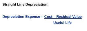
Therefore, in the case of MAAS Corporation, we can determine the yearly depreciation expense by dividing the depreciable base of $50000 ($65000-15000) by the economic life of five years, giving an annual depreciation expense of $10000. At the end of the financial year, MAAS Corporation will record the following entry:
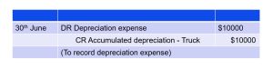
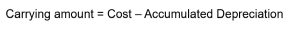
After the journal entry in year one, the truck would have a carrying amount (also called Net Value or Book Value or Written-down Value) of $55000. This is the original cost of $65,000 less the accumulated depreciation of $10000.
MAAS records an annual depreciation expense of $10000. Each year, the accumulated depreciation balance increases by $10000, and the truck’s book value decreases by the same $10000. At the end of five years, the asset will have a book value of $15000, which is calculated by subtracting the accumulated depreciation of $50000 (5 × $10000) from the cost of $65,000. This calculation is depicted in the depreciation schedule below:
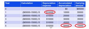
The depreciation schedule highlights three key things. First, depreciation expense is the same in each period. This will always be the case using the straight-line method. Second the accumulated depreciation account grows each year by $10000 until the balance equals the depreciable amount of the asset ($50000). A key takeaway here is the final balance in accumulated depreciation is the total of all depreciation expense recorded during the asset’s useful life and hence should equal the asset’s depreciable amount. Lastly, the carrying amount decreases by $10000 each year until it equals the residual value ($15000) estimated for the asset. Carrying amount represents the remaining unexpired cost of the asset and thus should always equal the estimated residual value at the end of the asset’s useful life.
Reducing-Balance Depreciation Method
The reducing-balance depreciation method is the most complex of the three methods because it accounts for both time and usage and takes more expense in the first few years of the asset’s life. It is an accelerated method that results in more depreciation expense in the early years of an asset’s life and less depreciation expense in the later years.
Reducing-balance considers time by determining the percentage of depreciation expense that would exist under straight-line depreciation. To calculate this, divide 100% by the estimated life in years. For example, a five-year asset would be 100/5, or 20% a year. A four-year asset would be 100/4, or 25% a year.
Next, because assets are typically more efficient and “used” more heavily early in their life span, the reducing-balance method takes usage into account by doubling the straight-line percentage. For a four-year asset, multiply 25% (100%/4-year life) × 2, or 50%. For a five-year asset, multiply 20% (100%/5-year life) × 2, or 40%.
 For tax purposes in Australia, reducing-balance at twice the straight-line rate is often used and referred to as the ‘double declining balance’ method. It is important to note that just because a business uses one method for taxation does not mean it has to use that method in its financial statements. This method may match expenses to revenues better than the straight-line method, because more depreciation expense is recorded when the asset is more useful but it also provide larger expenses (and if used for tax purposes larger tax-deductible expenses) in earlier years of a non-current asset’s life.
One unique feature of the reducing-balance method is that in the first year, the estimated salvage value is not subtracted from the total asset cost before calculating the first year’s depreciation expense. Instead the total cost is multiplied by the calculated percentage. However, depreciation expense is not permitted to take the book value below the estimated salvage value. Let’s better understand this through an example using MAAS Corporation. Let’s assume MAAS Corporation purchased a truck on 1st July for $65000. It has an estimated residual value of $15000 and a useful life of 5 years. The straight-line rate is 1/5 or 20 per cent.
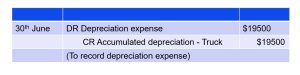
If we use 1.5 times the straight-line rate for the current year, depreciation would be [$65 000×(1.5 × 20%) = $19 500] and recorded as follows:
A depreciation schedule for all five years is shown below:
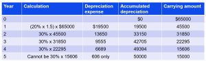
The depreciation schedule provides three key observations. First, there is more depreciation expense in the early years and less in the later years. Second, over an asset’s life, an entity cannot record more total depreciation than the asset’s depreciable cost. Notice that in the 5th year, the remaining carrying amount of $15606 was not multiplied by 30%. This is because the expense would have been $4681.80, and since we cannot depreciate the asset below the estimated salvage value of $15000, the expense cannot exceed $606, which is the amount left to depreciate (difference between the carrying amount of $15606 and the salvage value of $15000). Lastly, the depreciation rate is applied to the carrying amount of the asset. In this example, the first year’s reducing-balance depreciation expense would be $65000 × 30%, or $19500. Note that we ignore the residual value when calculating the depreciation expense. For the remaining years, the reducing balance percentage is multiplied by the remaining carrying amount of the asset. MAAS would continue to depreciate the asset until the carrying amount and the estimated salvage value are the same (in this case $15000).
The net effect of the differences in straight-line depreciation versus reducing-balance depreciation is that under the reducing-balance method, the allowable depreciation expenses are greater in the earlier years than those allowed for straight-line depreciation. However, over the depreciable life of the asset, the total depreciation expense taken will be the same, no matter which method the business chooses. For example, in the current example both straight-line and reducing-balance depreciation will provide a total depreciation expense of $50000 over its five-year depreciable life.
Units-of-Activity Depreciation Method
While the straight-line depreciation is efficient in accounting for assets used consistently over their lifetime, what about assets that are used with less regularity? The units-of-activity depreciation method bases depreciation on the actual usage of the asset, which is more appropriate when an asset’s life is a function of usage instead of time. For example, this method could account for depreciation of a truck for which the depreciable base is $50000 (as in the straight-line method), but now the number of kilometres the van is driven is important. Because units-of-activity relies on an estimate of an asset’s lifetime activity, the method is limited to assets whose units-of-activity can be measured.
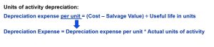
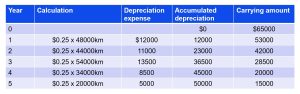
Let’s return to the example of MAAS Corporation and the truck it purchased for $65000 on 1st July. It has an estimated residual value of $15000 and a life of 200000 km. This means that the truck will have total depreciation of $50000 over its useful life of 200000km. Thus,
Depreciation per km is $0.25 per km ($65000 – $15000) ÷ 200000.
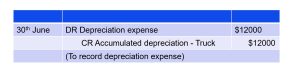
If the truck is driven 48000 km in the current year, depreciation expense would be $0.25 per km x 48000 km, or $12000, and recorded as follows:
The journal entry to record this expense would be the same as with straight-line and reducing-balance depreciation: only the dollar amount would have changed. The presentation of accumulated depreciation and the calculation of the book value would also be the same. MAAS would continue to depreciate the asset until a total of $50000 in depreciation was taken after the truck travelled a total of 200000 (48000+44000+54000+34000+20000) km, as depicted in the depreciation schedule below:
Summary and comparison of depreciation methods
The table below compares the three methods discussed. Note that although each method’s annual depreciation expense is different, after five years the total amount depreciated (accumulated depreciation) is the same. This occurs because at the end of the asset’s useful life, it was expected to be worth $15000: thus, all three methods depreciated the asset’s value by $50000 over that time period.
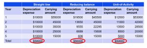
However, each method arrives at the $50000 differently. The straight line method depreciates the same amount ($10000) each year. The reducing balance method accelerates depreciation into the early years of the asset’s life. The units of activity method depreciates different amounts annually depending on the asset’s usage. No method is right or wrong, just different. Businesses choose a method for different reasons, including tax benefits, to report the ‘best’ profit number, and so on. Regardless of the method chosen, businesses should disclose their choice of depreciation method in the noted of their financial statements so that comparisons can be made among different companies. As seen in Section 7.1, the disclosure is usually provided in a note related to PPE (as shown in the Westfarmers example in Section 7.1).
When analysing depreciation, accountants are required to make a supportable estimate of an asset’s useful life and its salvage value. Accountants need to analyse depreciation of an asset over the entire useful life of the asset. As an asset supports the cash flow of the business, expensing its cost needs to be allocated, not just recorded as an arbitrary calculation. An asset’s depreciation may change over its life according to its use. If asset depreciation is arbitrarily determined, the recorded gains or losses on the disposition of depreciable property assets (covered in Section 7.4) seen in financial statements are not true best estimates. Due to operational changes, the depreciation expense needs to be periodically reevaluated and adjusted. We now turn our attention to understanding the effects of adjustments that may be made during a non-current asset’s useful life.
